Hey, 

After weeks of trying to deconstruct Paul's next stage of the Flower setup, I've managed to figure it out, at least most of the Nodes, and I'm happy to share my thinking process with you.

However, I think this setup could be slightly modified so that it's easier to update the Petals and produce a brand new flower.

Some Attribute wranglers used a lot of math. However, VEX could be simplified or even removed at all in a few nodes, at the same time keeping the original procedural setup.

Below, you will find a step-by-step development of a still composition of a flower, which later will be used as a starting point for the Vellum Simulation. If you spot any mistakes or you might have suggestions please feel free to reach out.

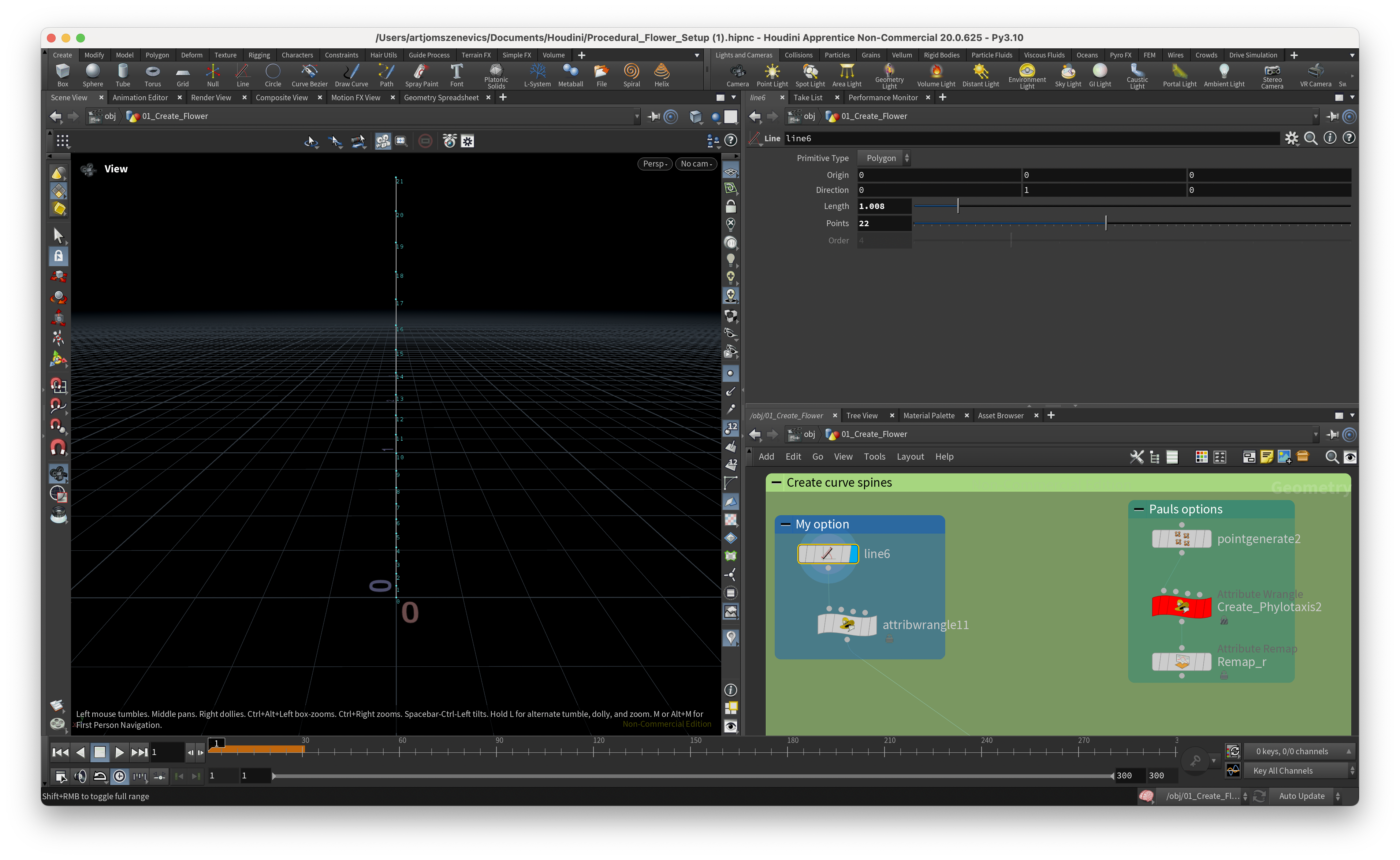
Step 1.

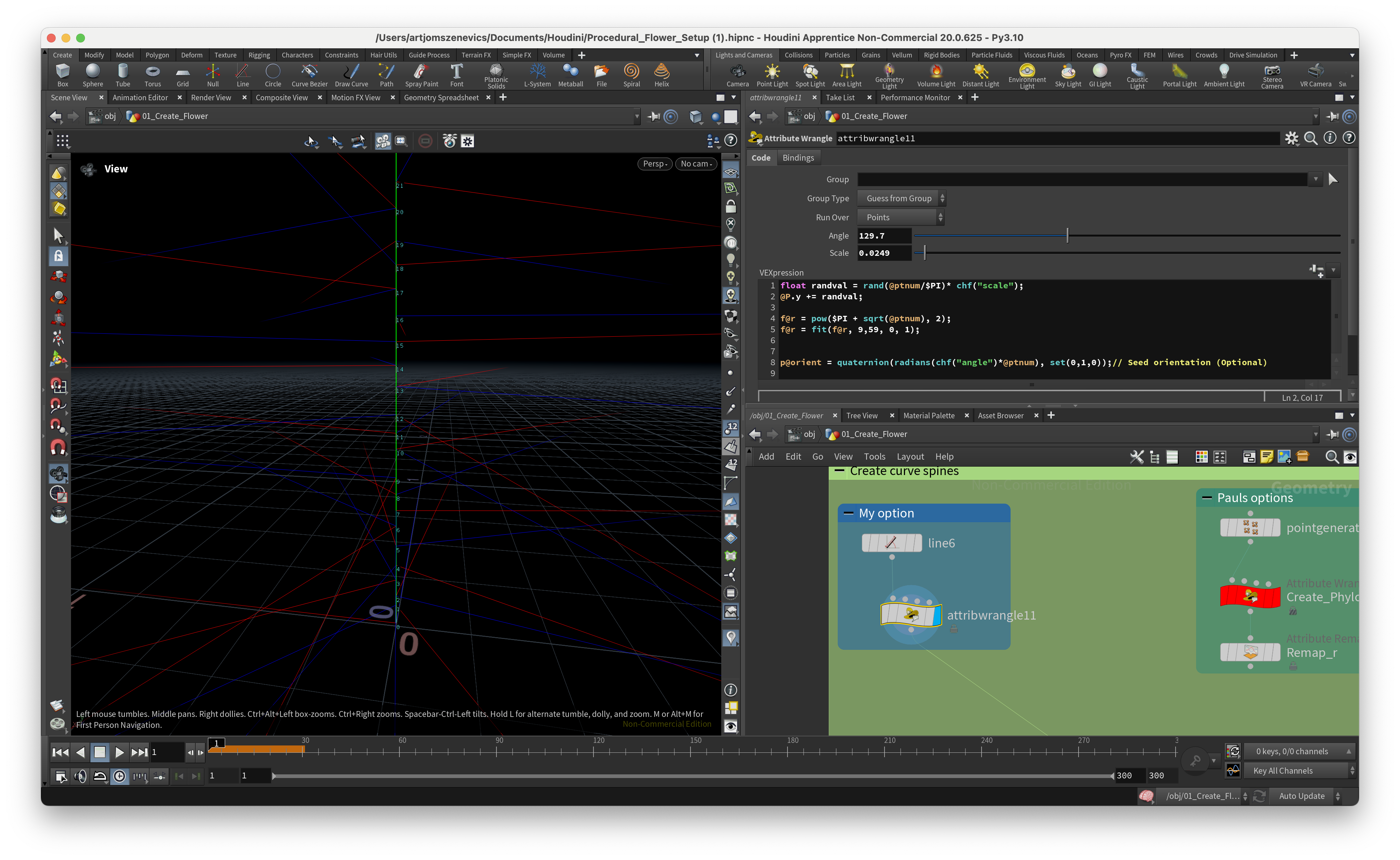
Paul uses complex VEX script to distribute the points. It basically gives you a lot of controls and, in addition, he also assigns a few extra attributes such as quaternion (p@orient) and float “r” value (f@r).

In my case, I wanted to keep things clean and simple so I’ve just decided to create a “Line” node with the same amount of points (However later in the process I’ve realised that some flowers required more petals thus more points on the line)and create an individual attribute wrangle to assign p@orient(quaternion) and f@r values separately. These variables will be later used to control the distribution and bending of petals.

The only thing is that I’ve added extra line:

float randval = rand(@ptnum/$PI)* chf("scale");

@P.y += randval;

And it’s going to shift randomly each point by Y axis. This will give us a very small organic feel when we’re going to copy the petals onto the Y axis.

Step 2.

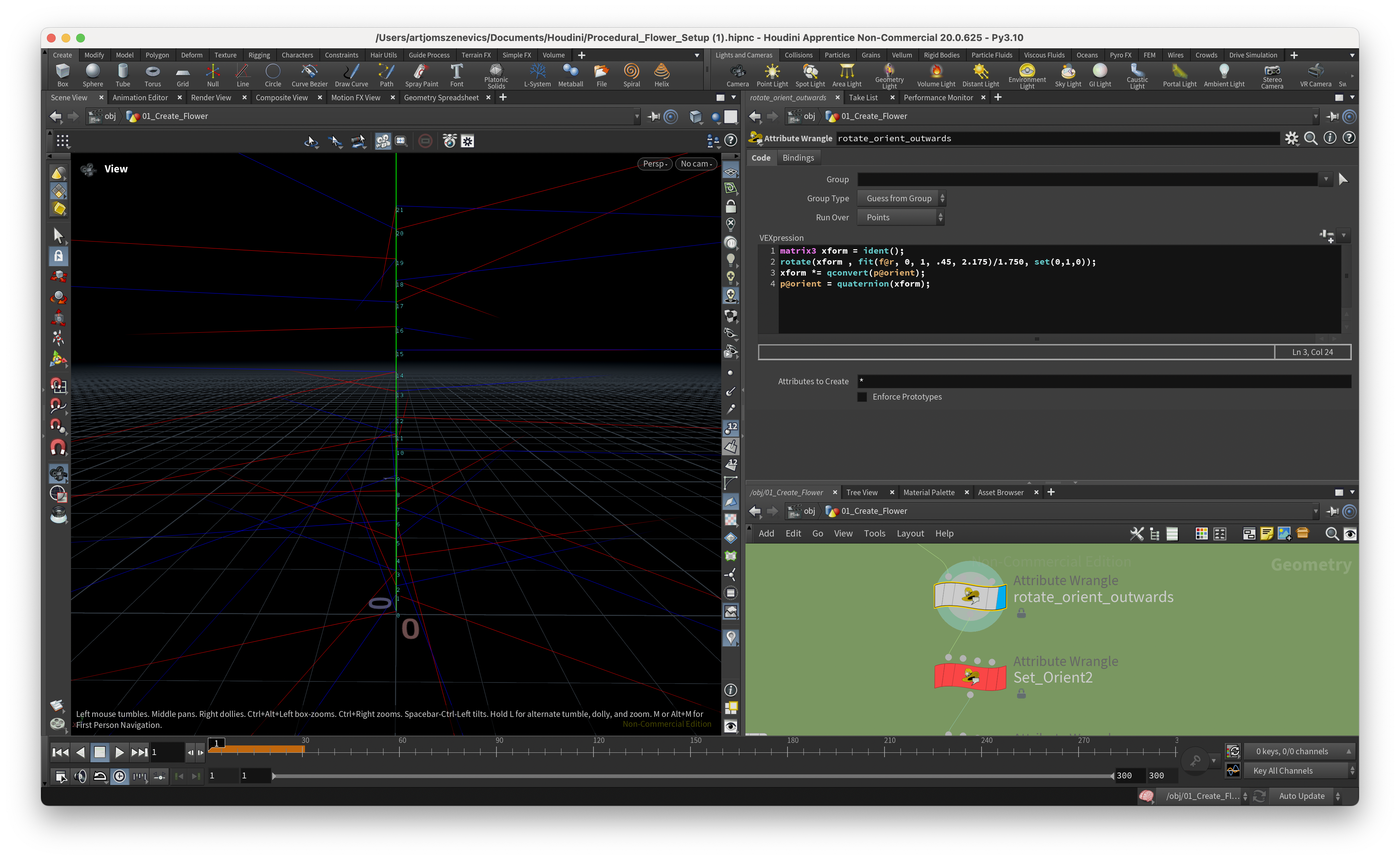
Next VEX code was quite complicated for me since Paul didn’t explain the VEX code much rather simply telling what its going to be the output. Ultimately, what this node does is shift slightly our previously defined p@orient attribute. Paul uses here rotational matrix here to rotate the points and then converts back to the quaternion.

As I’ve mentioned earlier I’ve decided to keep things simple and I’ve noticed if we turn off this node then it doesn’t change the output much.

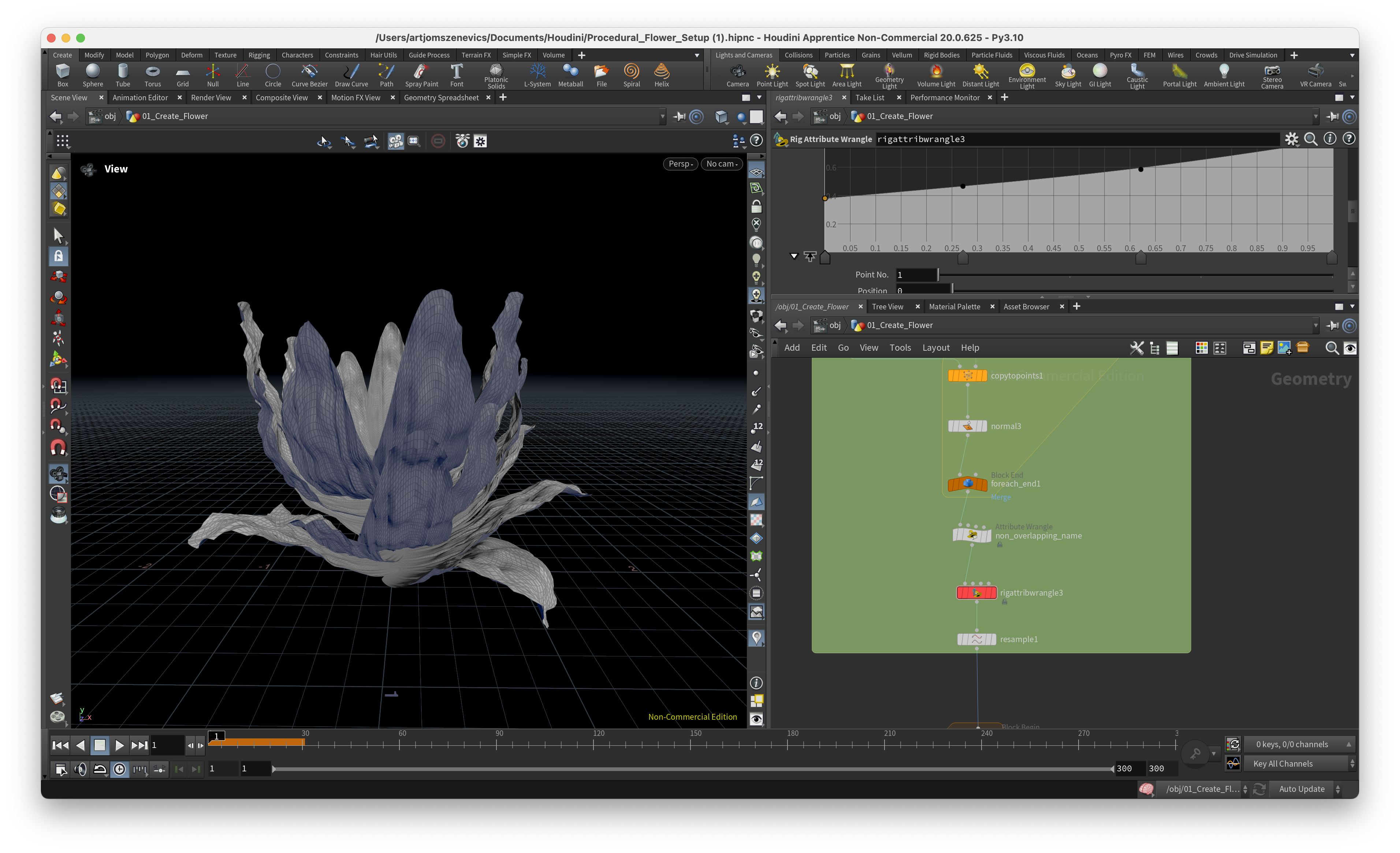
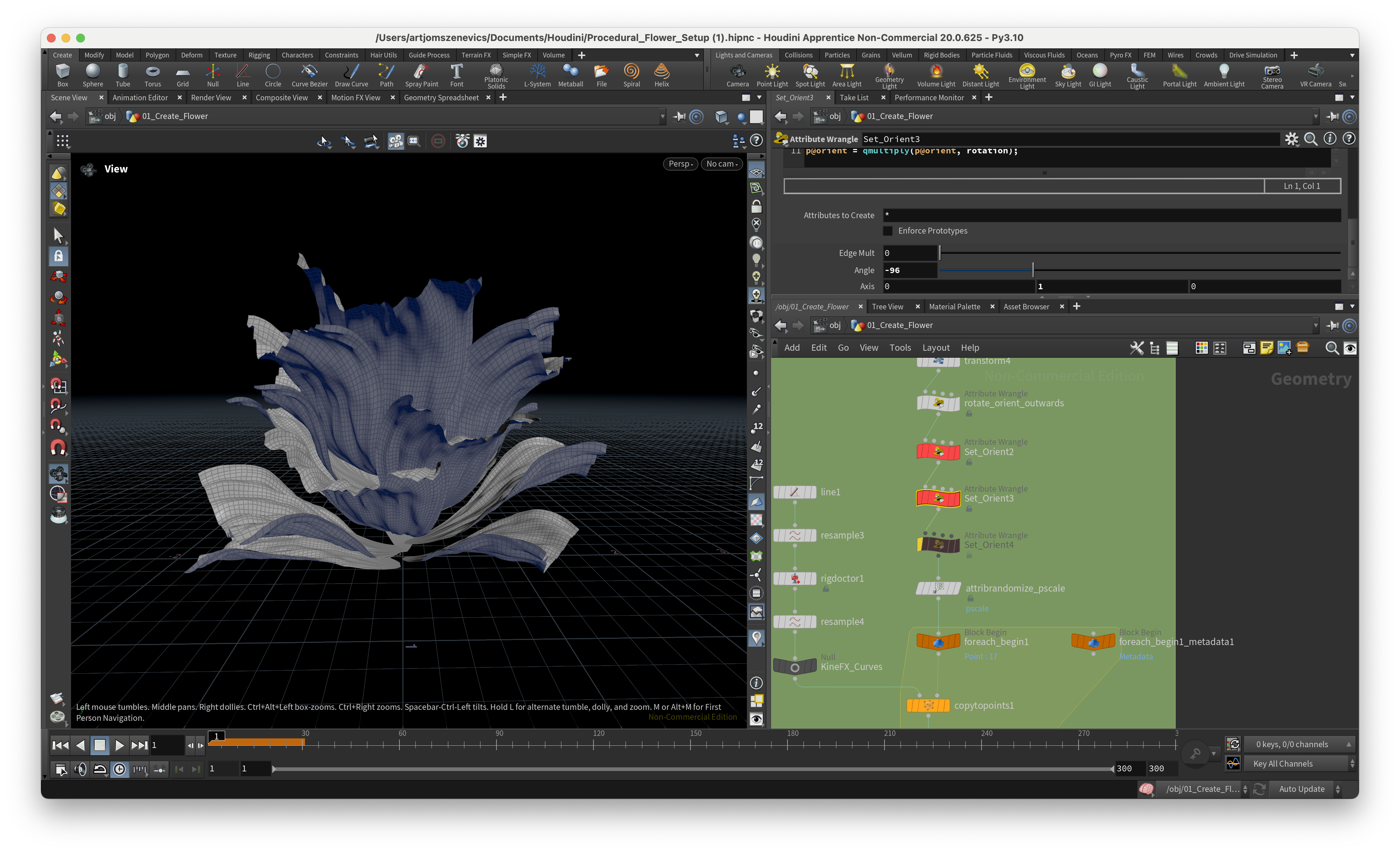
Step 3.

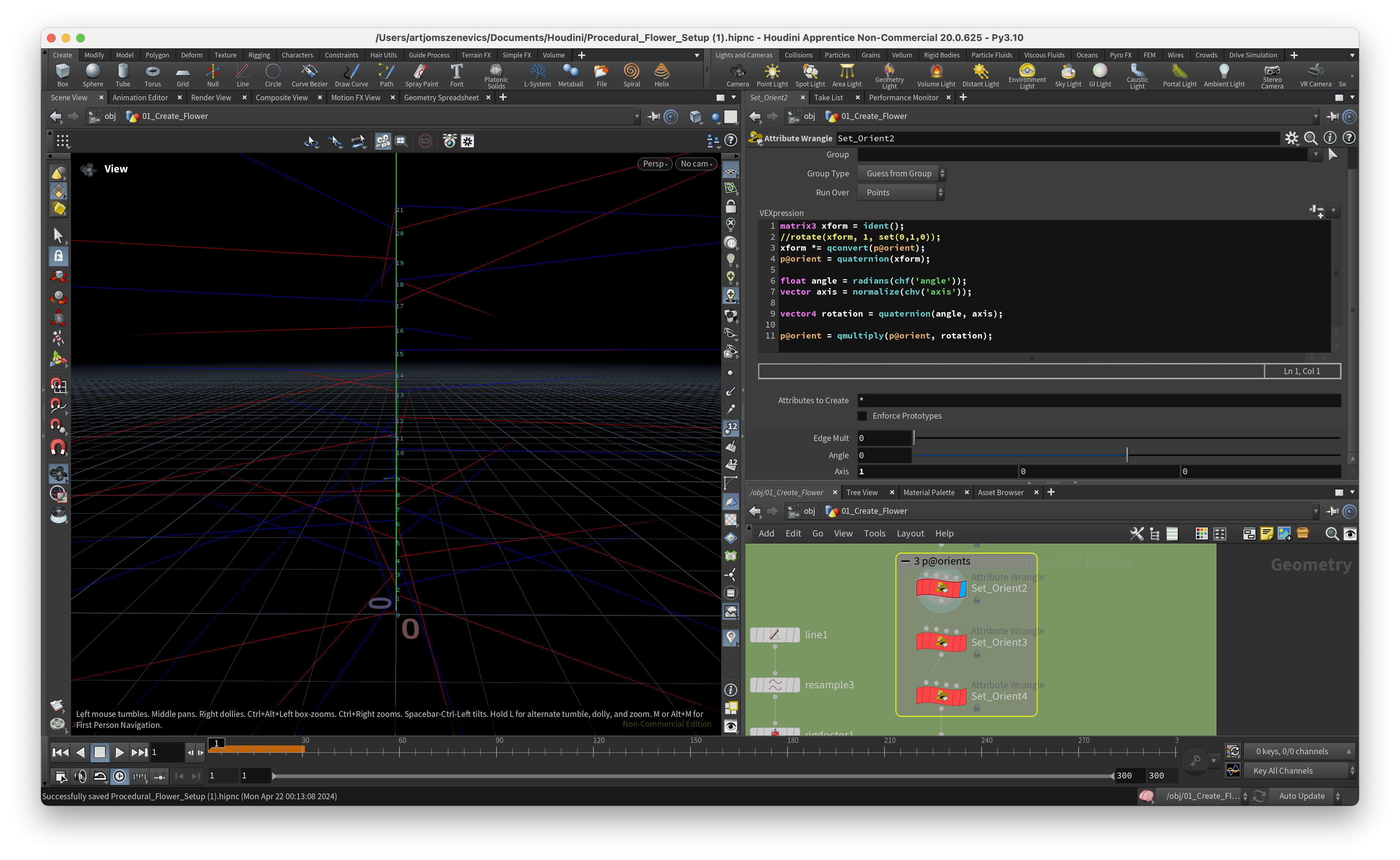
Here I will cover 3 nodes in a row because what each Node does is change the angle for our p@orient attribute, which gives us good control over our petal rotation. But each Node has it’s own p@orient attribute which was very confusing for me at first.

The key takeaway from here was my understanding of how quaternions work. In short, a quaternion is a four-dimensional vector that can be used to rotate objects in three-dimensional space. In Houdini, to create a quaternion we can apply the quaternion() function and inside we need to specify the axis + angle (radians). The axis can be created by set(0, 1, 0) and the angle can be done as a converted to radians channel float attribute radians(chf(”Angle”)).

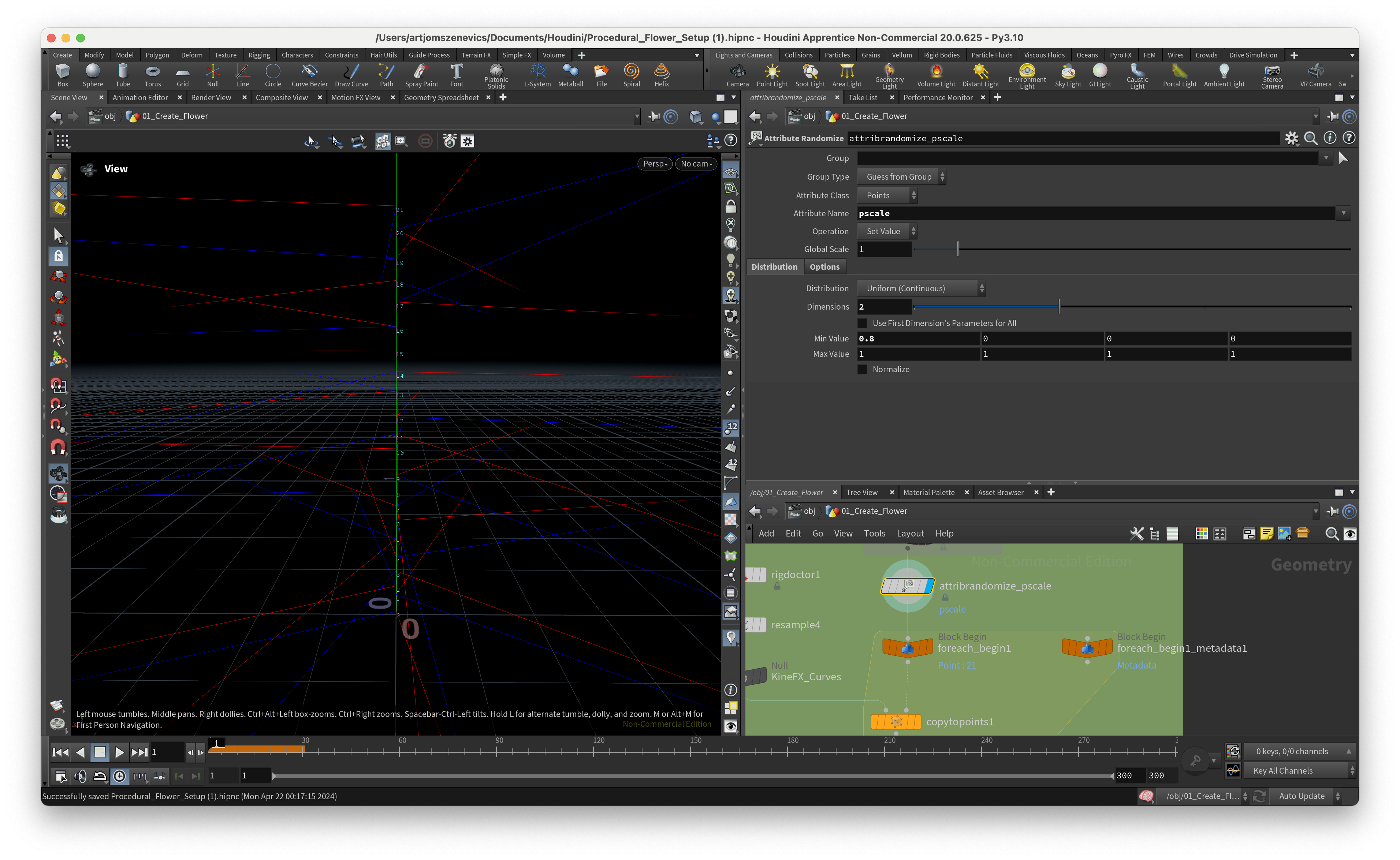
Step 4.

Next, we create an attribute Randomize Node and here we would like to slightly randomize the scale attribute, which will determine our petal size after we clone our petals. In short, the pscale attribute controls the size of your geometry. And with pscale, you can uniformly control the size of particles and points. In our case, we’ve randomized our pscale attribute from 0.8 to 1. Meaning the size of our petals will vary only by 20%, which will give us a nice organic difference in size.

Step 6.

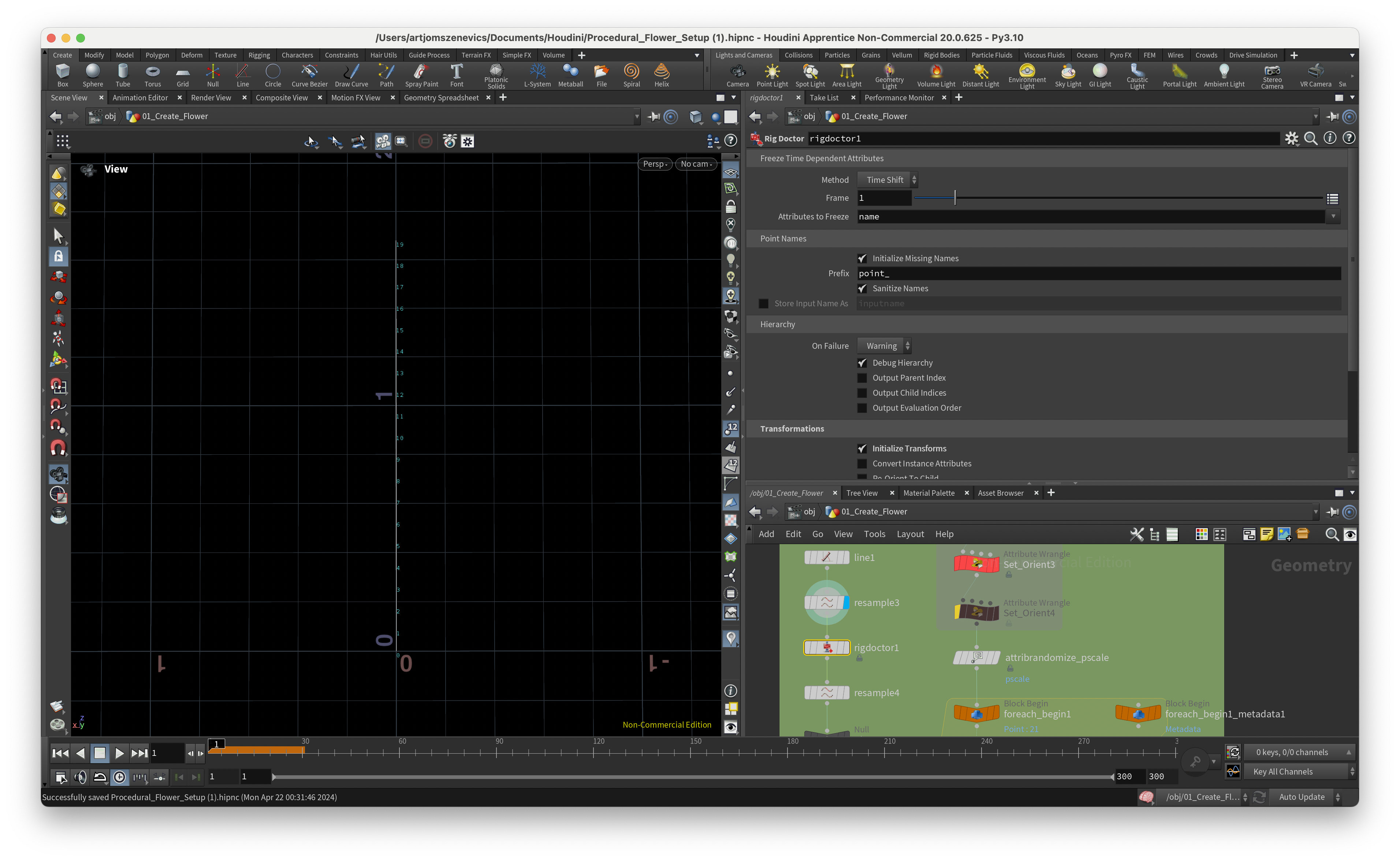
The next stop is about KineFX in Houdini and there are the rigging frameworks. The “Rig Doctor” Node will help us to do a few things:

1. Assigns a 4x4 matrix which will define our line behavior.

2. By modifying matrices with prerotate(), we will be able to change the curves.

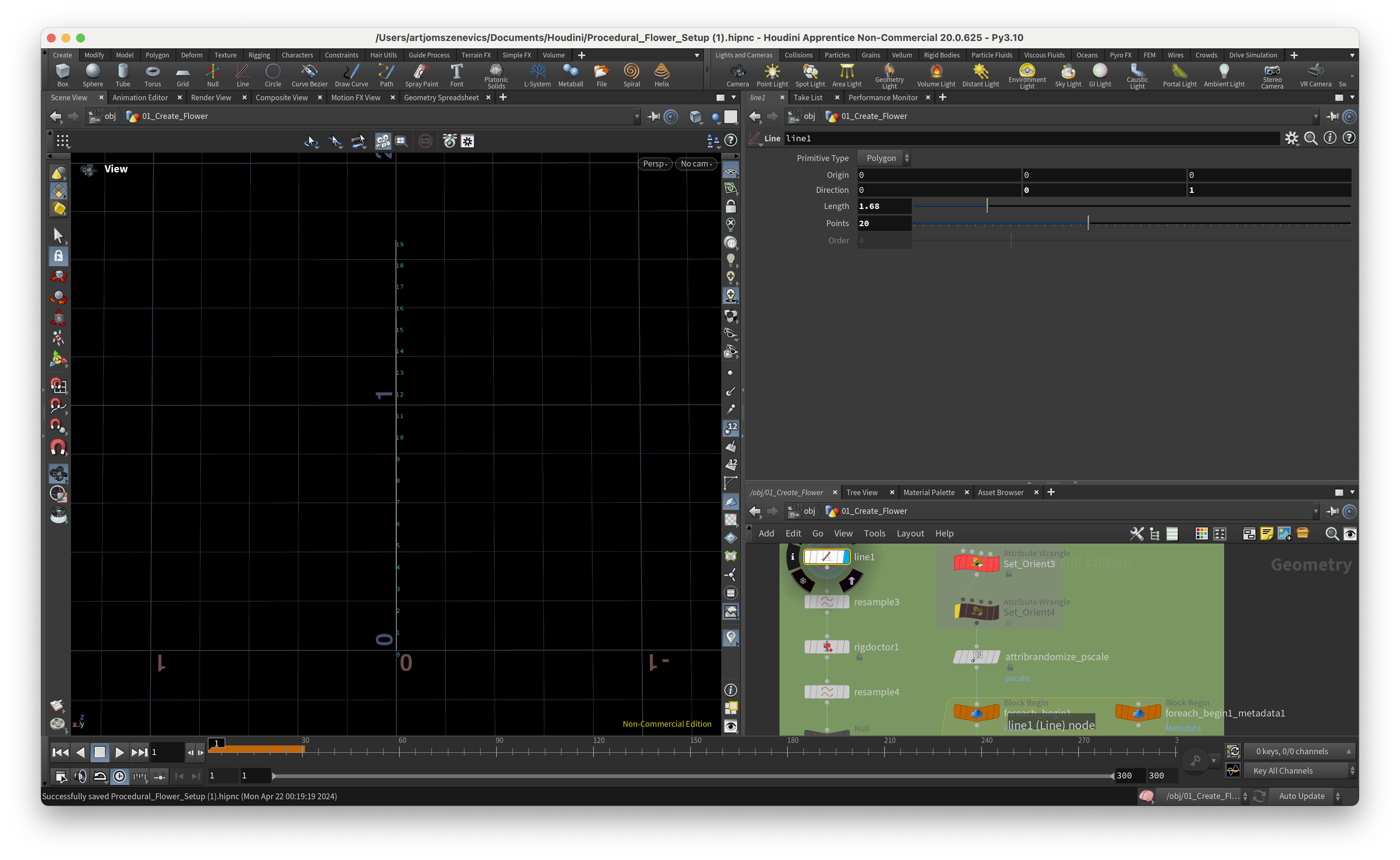
To start, we will create a Line with 20 points. Adding a Resample node and assigning it the curveu attribute, which later we will be using inside of chramp(). Next, we’re adding a “rig doctor” node and inside we would like to initialize the name “point_” and put a checkmark on “Initialize Transform”.

Step 7.

This is very confusing still to me why do we need to put the KineFX lines into the foreach loop when we can simply input straight into copy to points. ANYWAYS. I’m going to stick to Paul's process just to go through his pipeline. So, the copytopoints Node will go inside the foreach loop. And KineFX line will be inserted in the 1st geohandle. 

And, we’re adding a Normal node which will make our polygon mesh smoother.

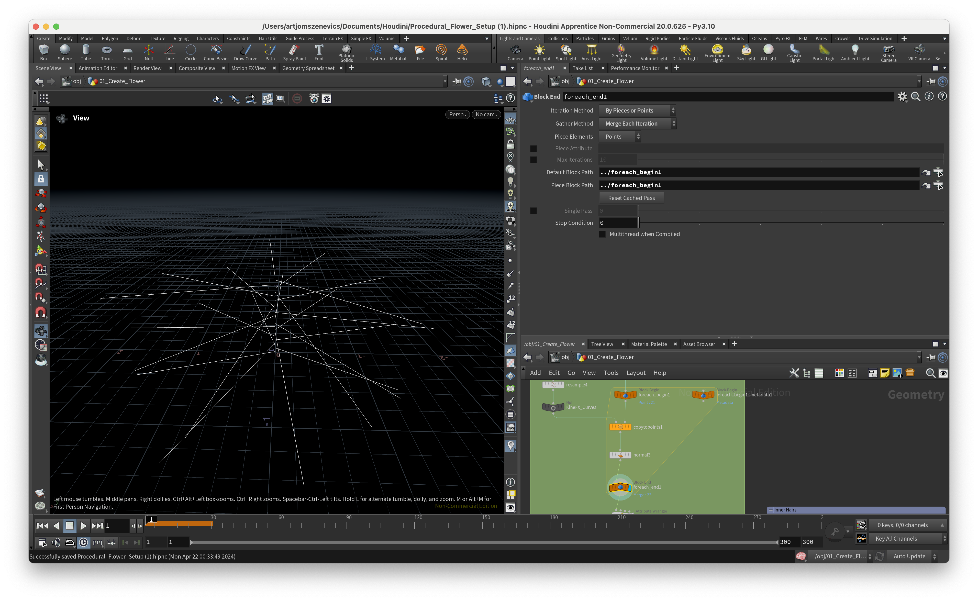
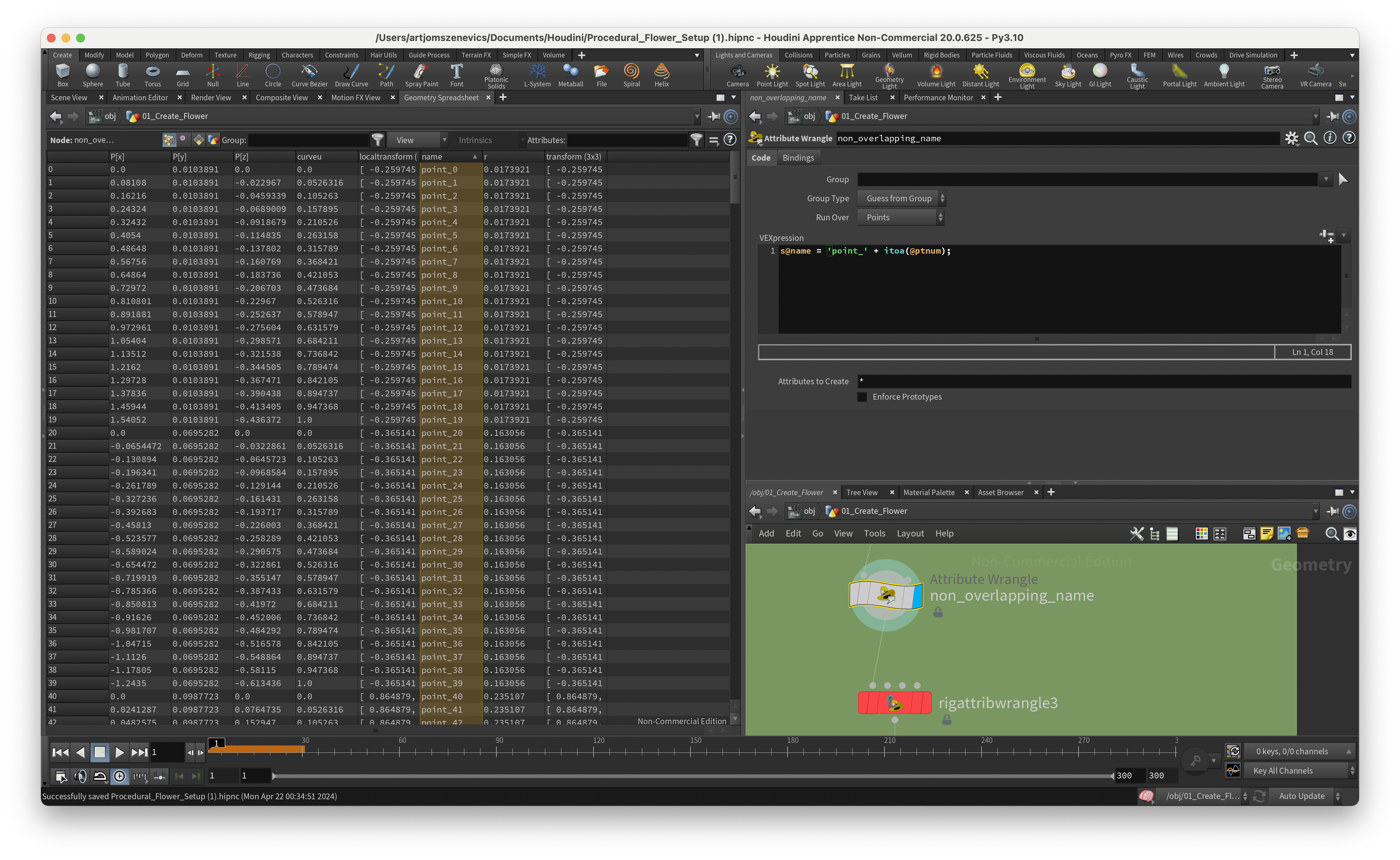
Step 8.

After we’ve cloned our lines on our points we would like to transform the local matrix which will end up in changing the curve. But before that, we would like to update each point's “name” variable with a unique name. This will help us to avoid any errors in the future. We are going to replace the current name with “point_” and the current point number.

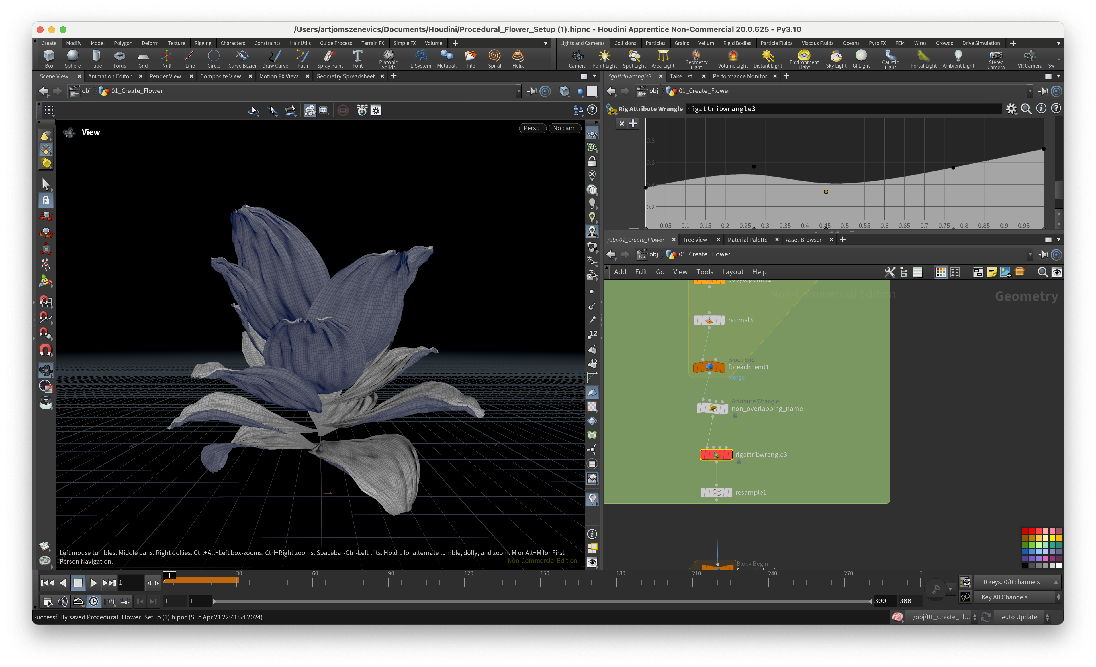
Step 9.

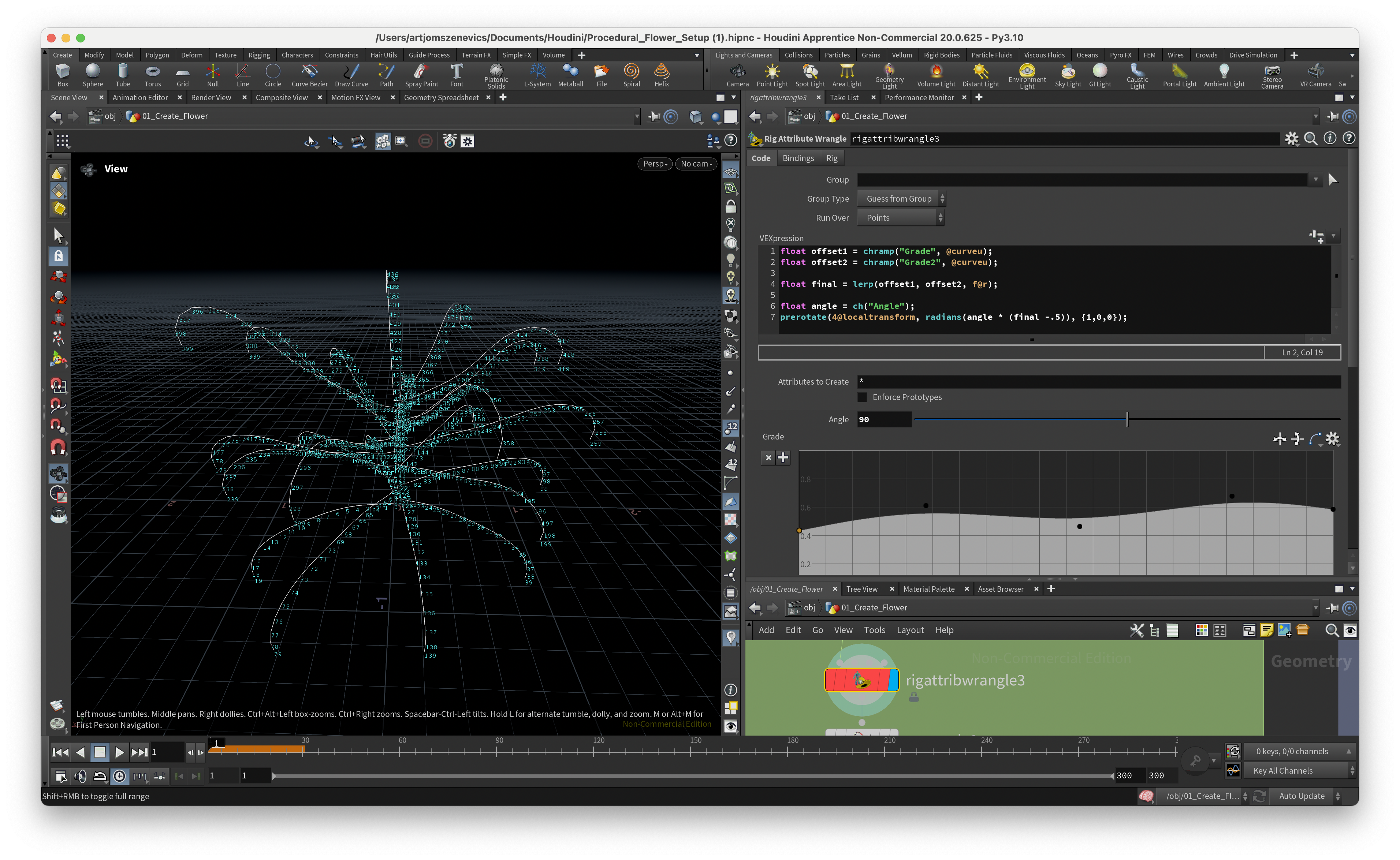
This step is about applying all of our previously created curve attributes in combination with linear interpolation. 

float offset1 = chramp("Grade", @curveu);

float offset2 = chramp("Grade2", @curveu);

float final = lerp(offset1, offset2, f@r);

float angle = ch("Angle");

prerotate(4@localtransform, radians(angle * (final -.5)), {1,0,0});

By modifying the 1st Ramp we are affecting the top part of curves. And by modifying the 2nd Ramp we are affecting the bottom curves.

However, these both Ramps are affecting one another because of the ”r“ attribute which we’ve distributed along our line. (I think I’ve spent a week to understand this part here) Meaning if the “r” value is 0 then on the output we will receive the offset1. And if the “r” value is 1 then we will have the output of offset2.

At this stage, I’ve decided to test how ChatGPT will interpret this line for me and this is what he said:

“In simple terms, this code takes two values from value ramps, blends them based on another value, and then rotates something based on the result and a user-defined angle. The rotation occurs around the x-axis, and how much it rotates depends on the blended color and the user-defined angle.”

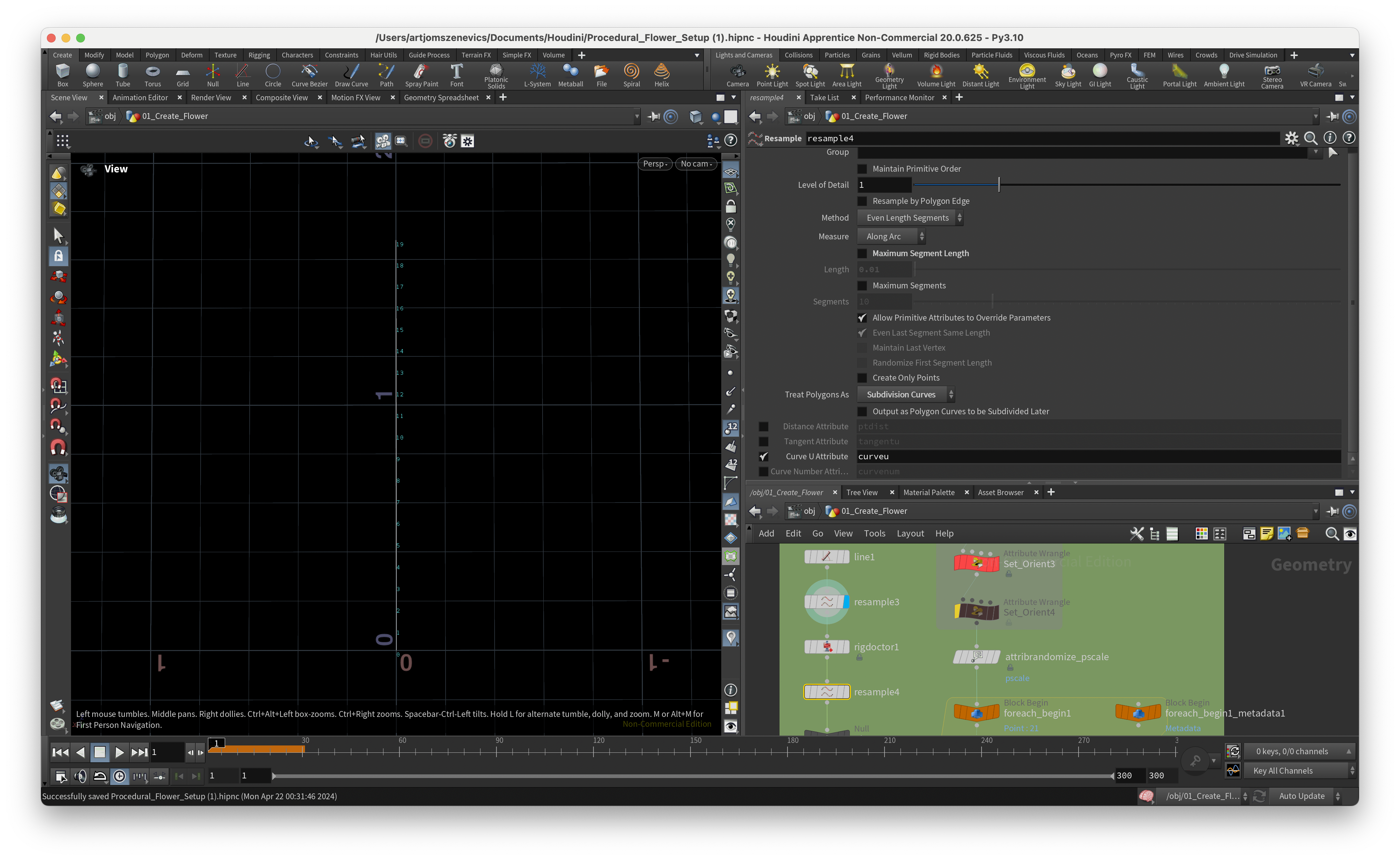
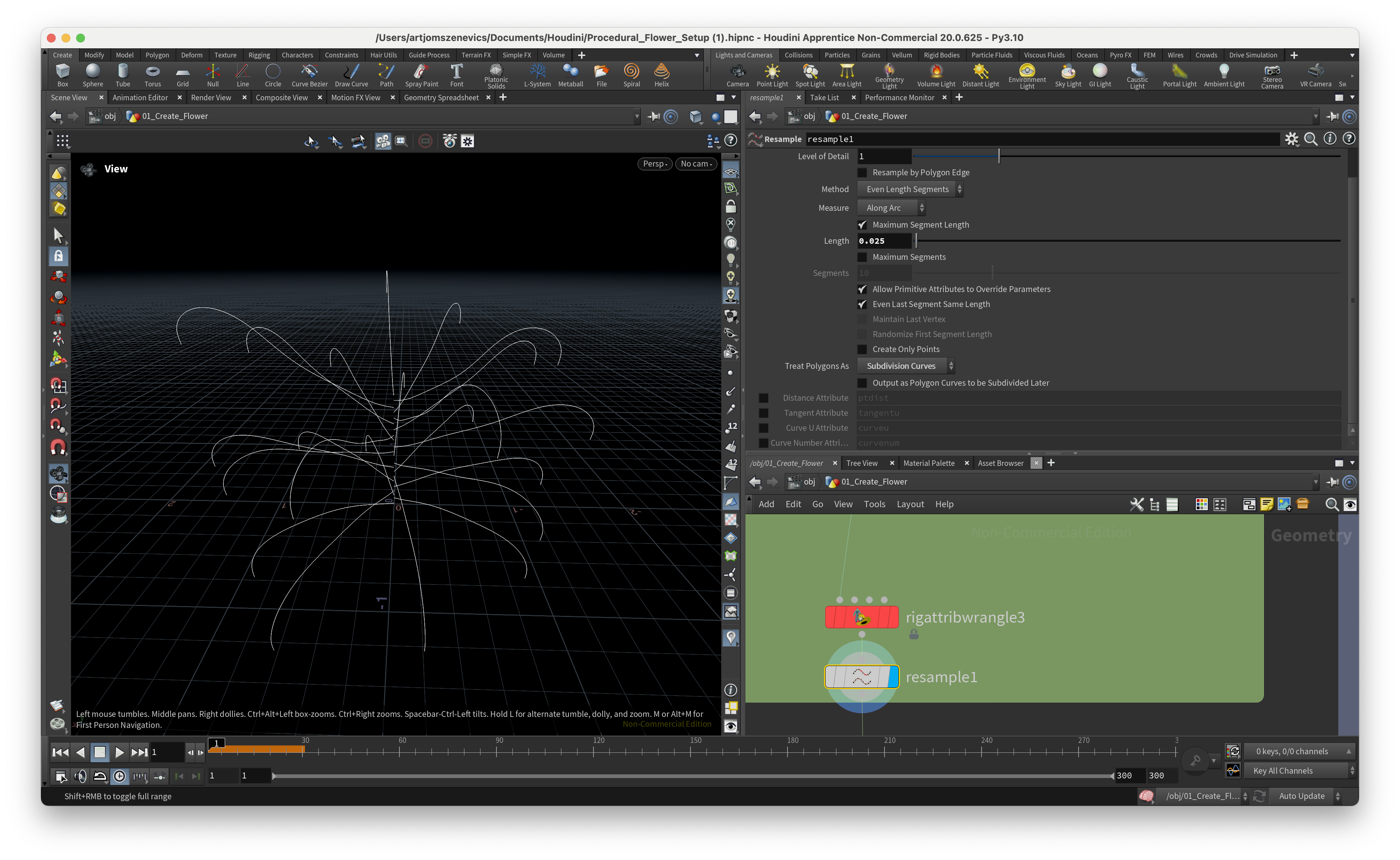
And to wrap up this section we’re applying a resample node to increase the number of points that we have on the line.

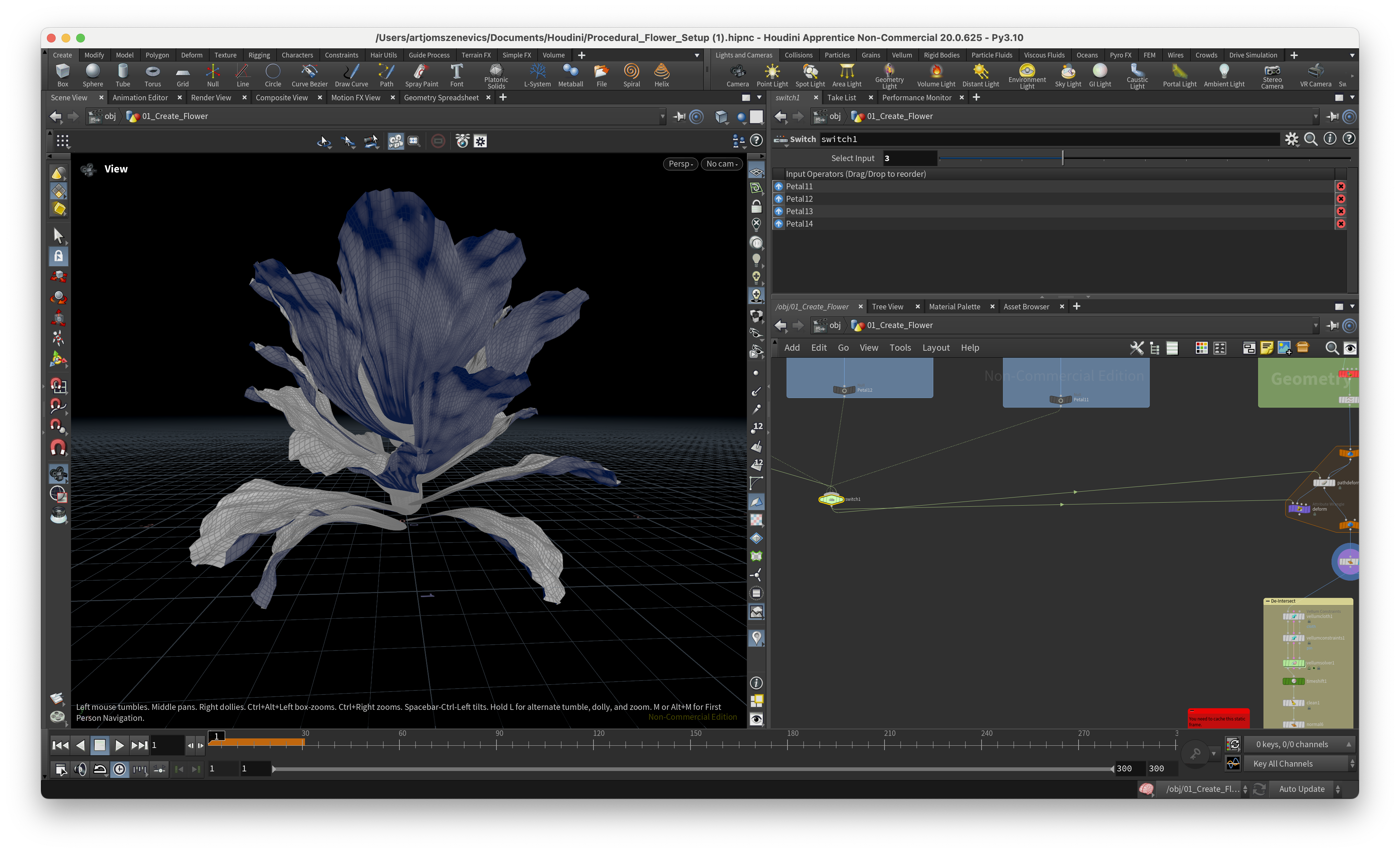
Step 10.

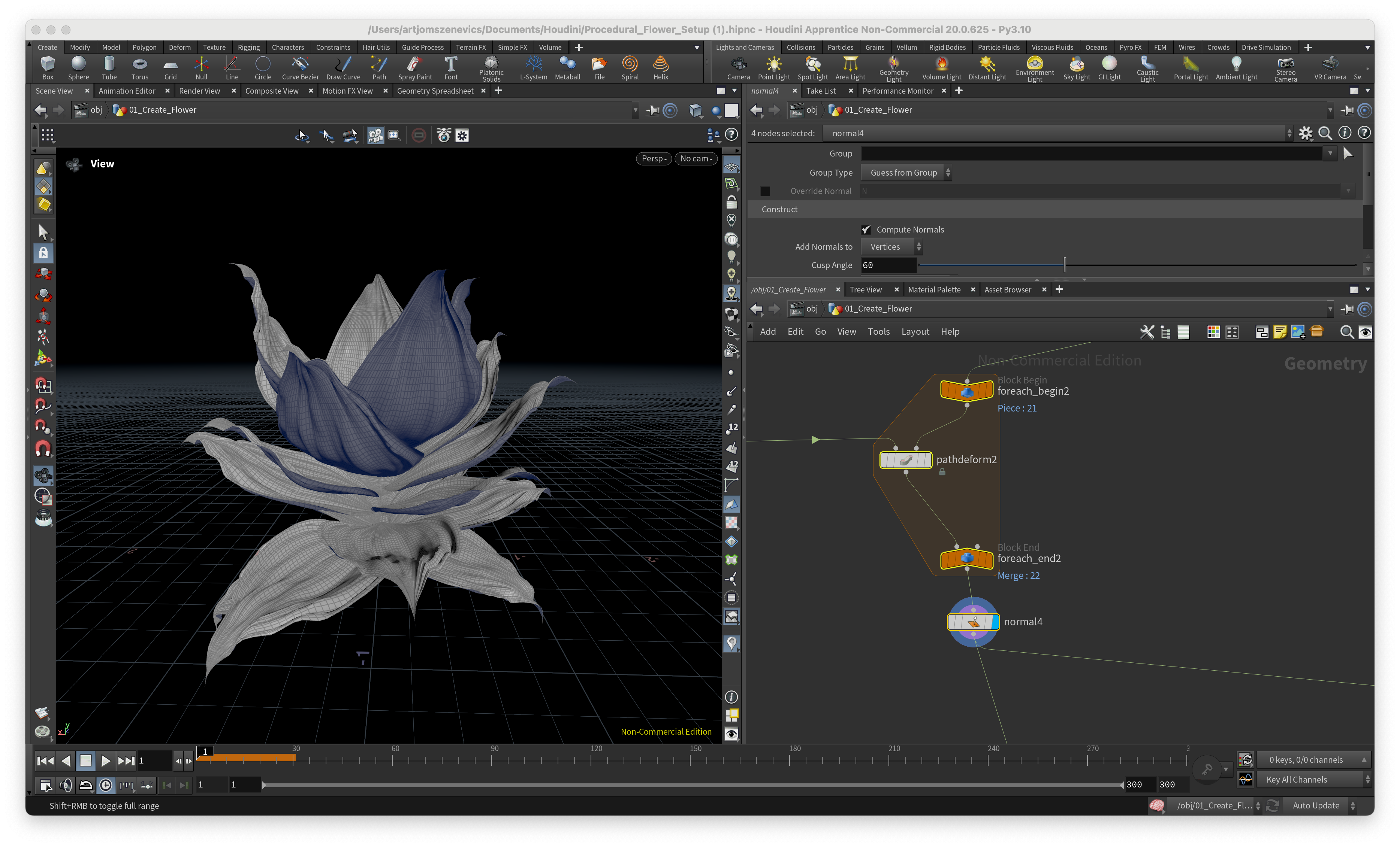
Finally, now we can distribute petals that I’ve created in the previous step and play around with different ramps to make sure we don’t have any intersections in geometry. It is very important to input non-intersecting geometry into the vellum solver. So inside the For loop, we insert a “path deformer” node which will deform our petals across the curves. For some Reason Paul wasn’t able to figure our how to not get errors with this Node but I’ve managed to find that the option “Fraction of Curve Length” managed to do the trick. Next section is going to be dedicated to the creation of a pistil which later is going to be placed in the center of our flower.

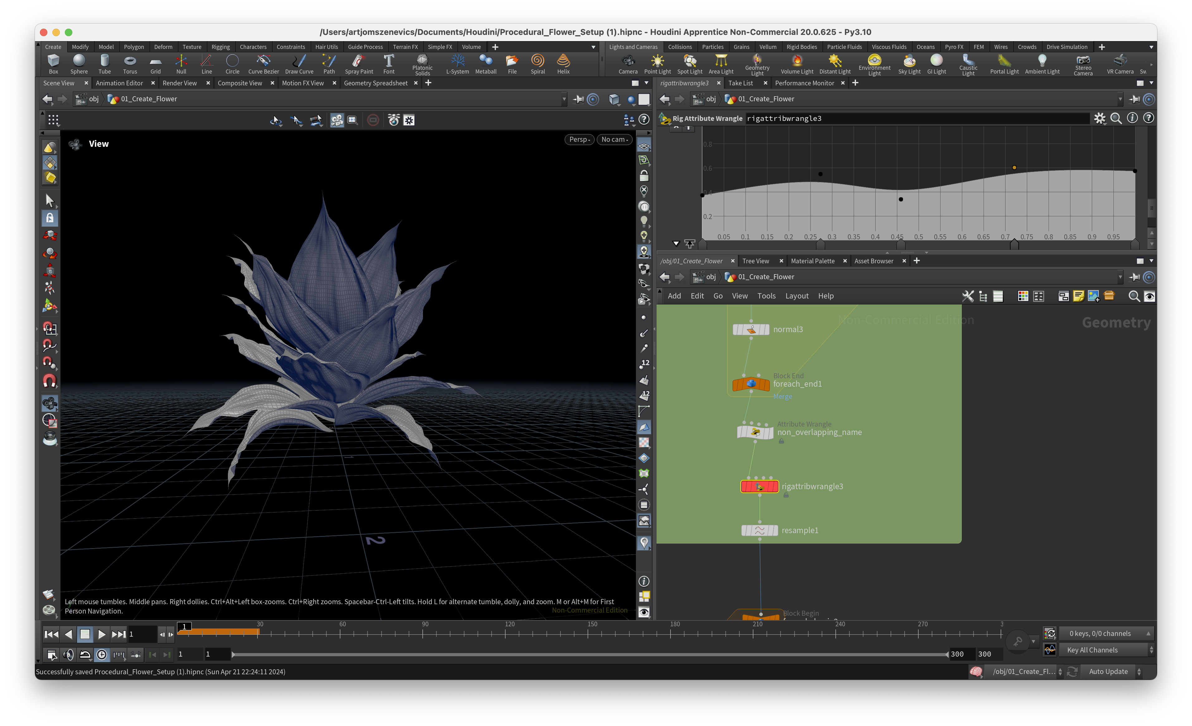
Conclusion: I had a lot of difficulties in understanding all the VEX code but key take aways for me is that quaternions and rotational matrixes are very useful when writing custom Attribute wranglers. 

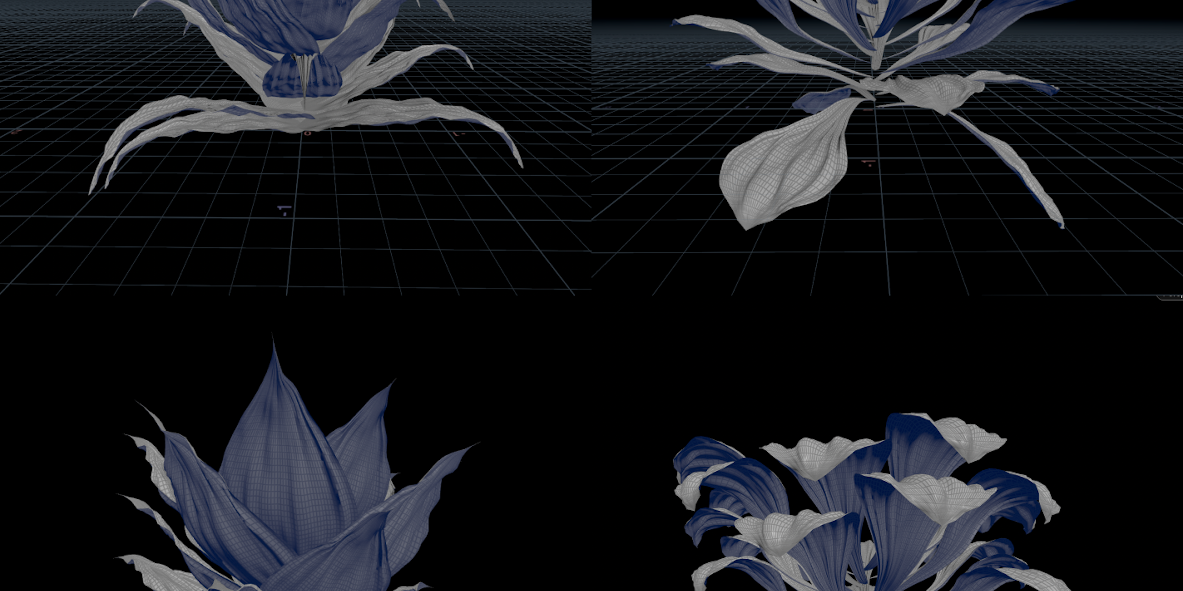
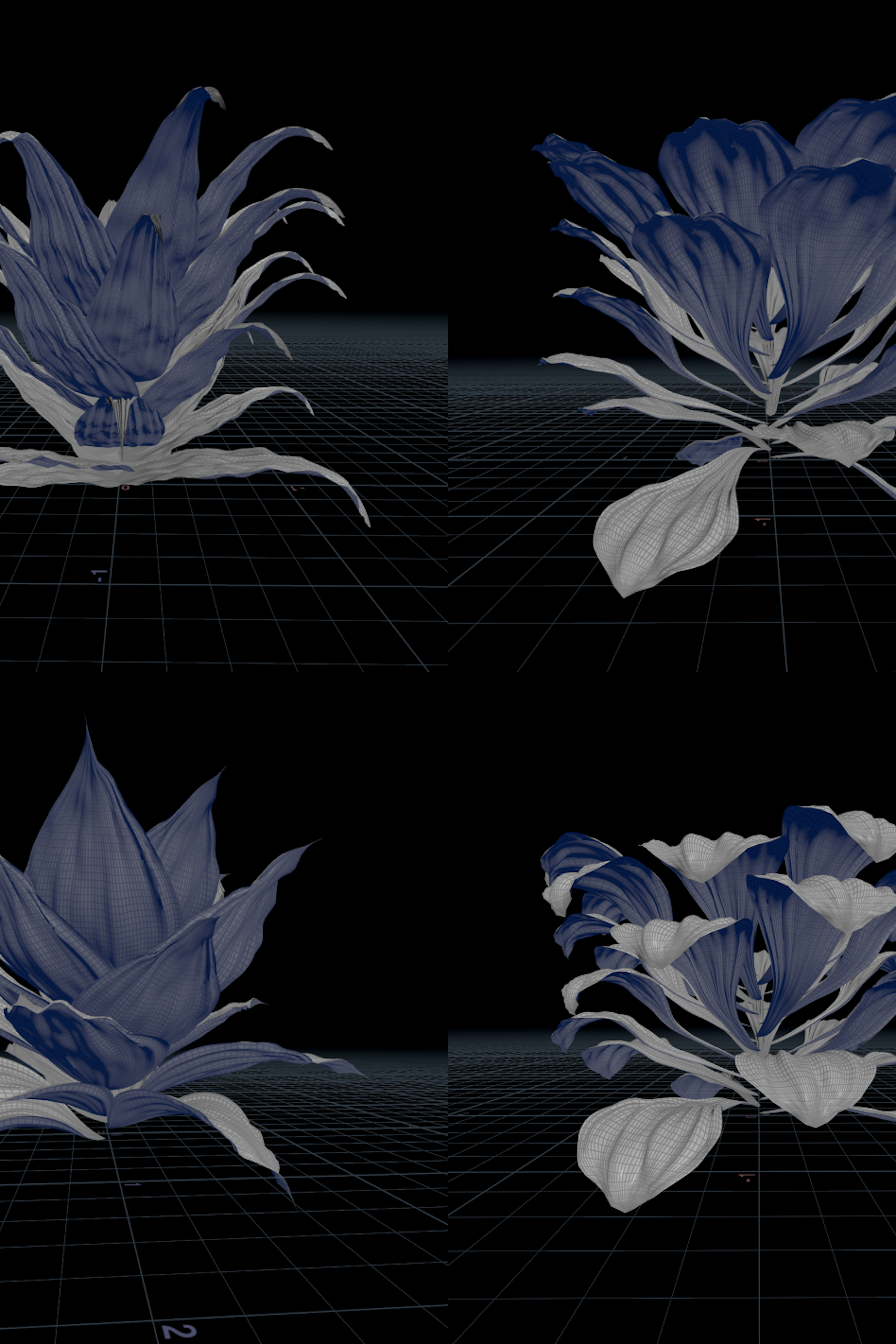
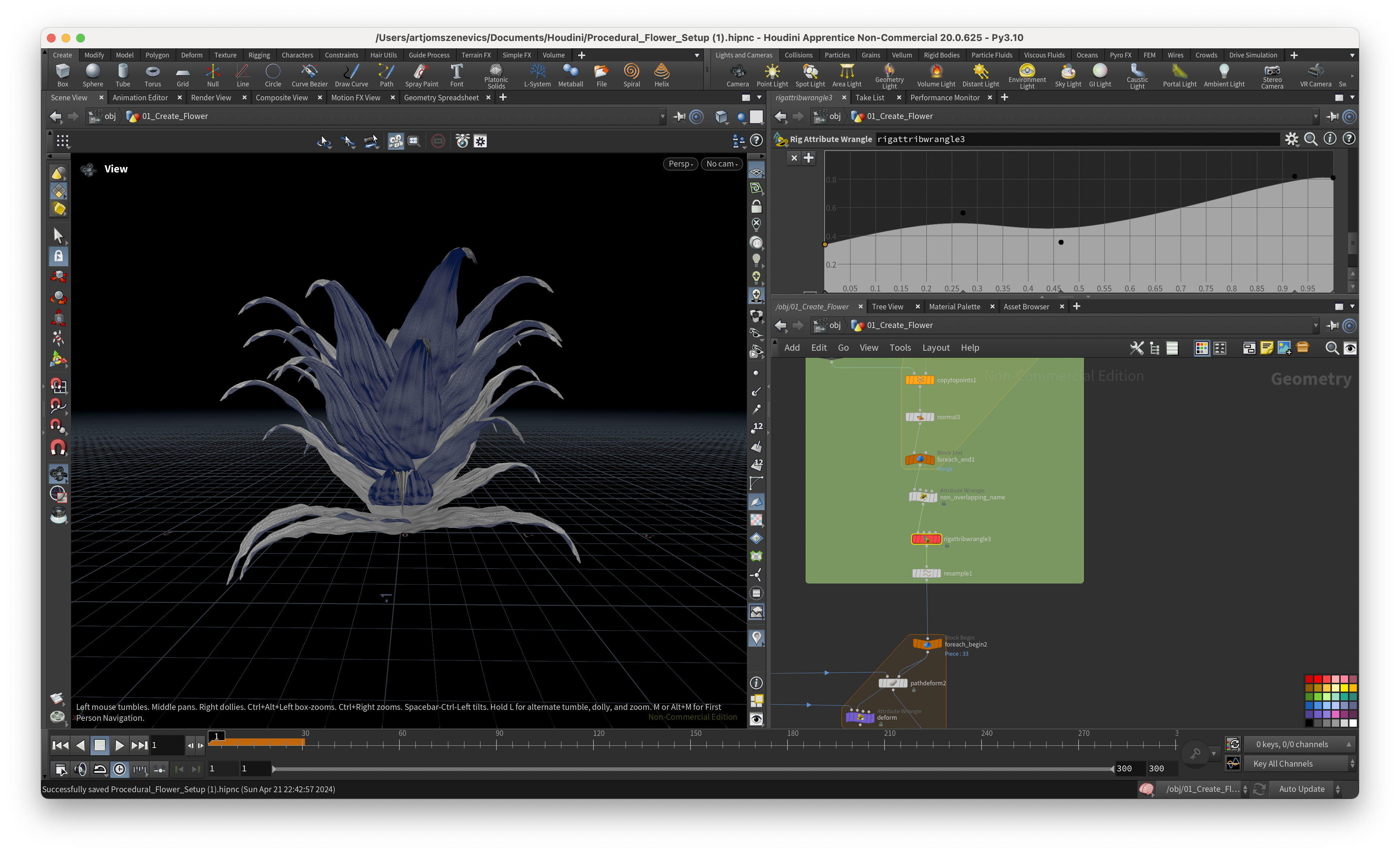
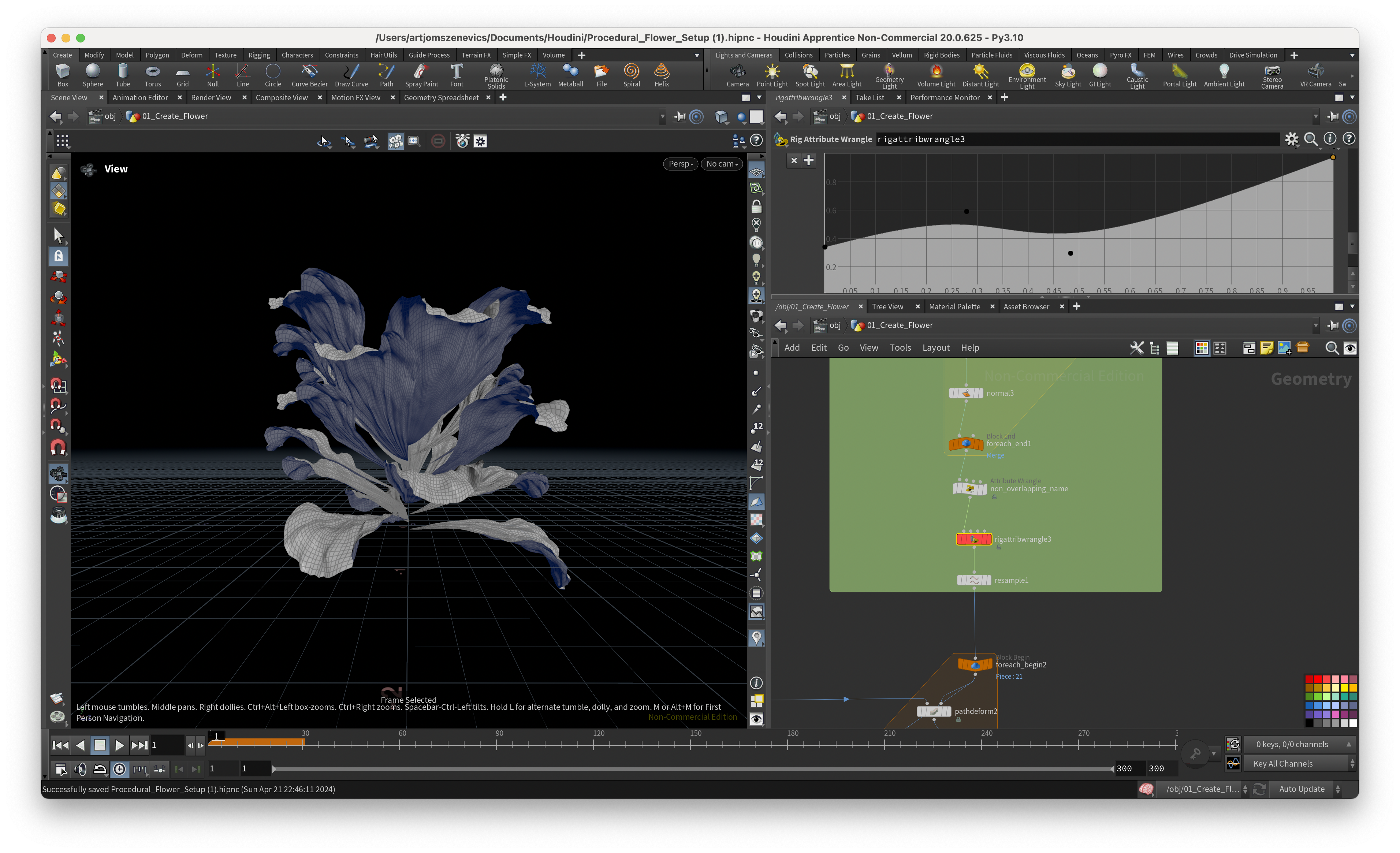
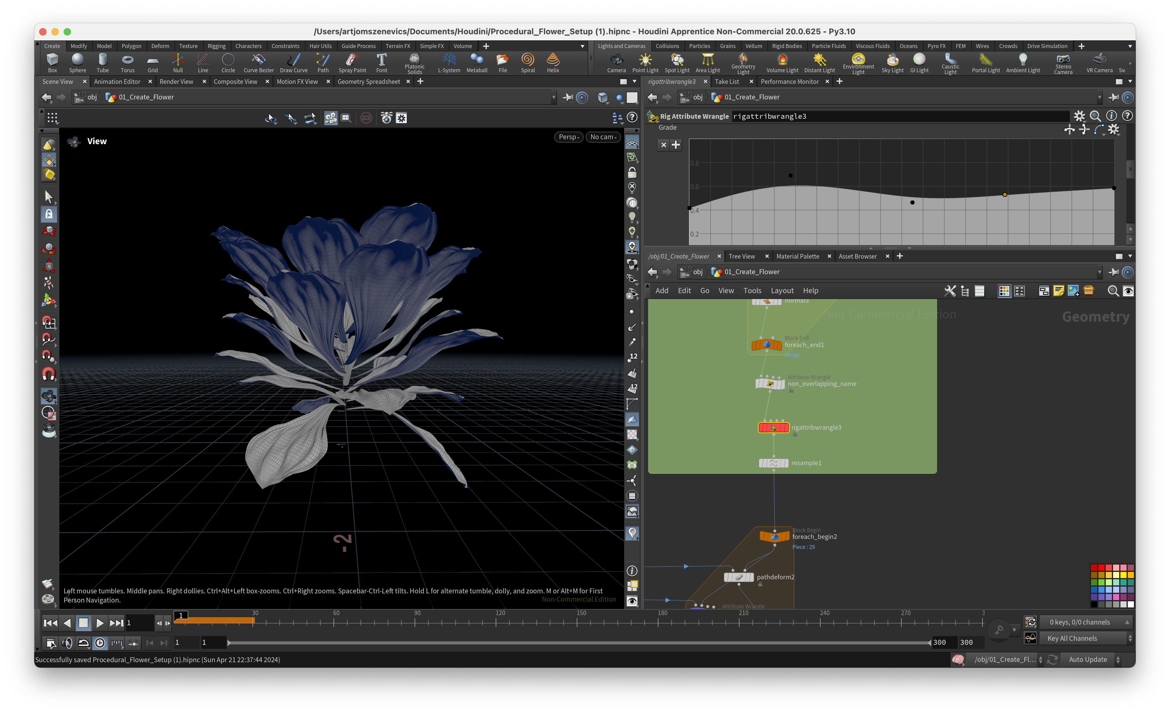
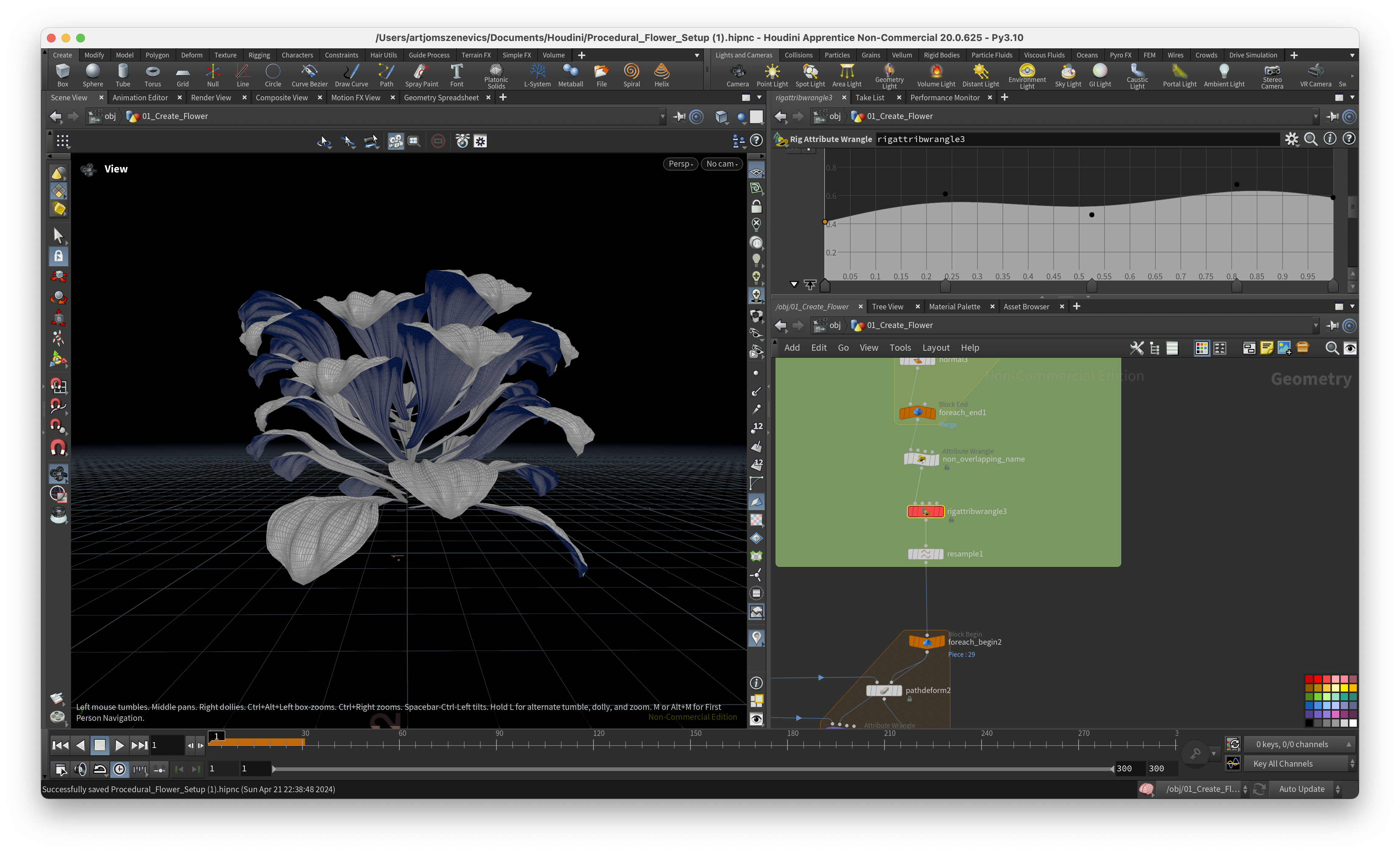
And here are some of the results of static flower which I was able to achieve using Pauls setup. Some are good but some came out quite weird: 

Next, the section is going to be dedicated to the ccreation of a pistil which will later be placed in the center of our flower.