Hi,
My third part will be entirely dedicated to the For Each loop and Vellum simulation. I find it quite difficult to grasp the long chain of nodes with VEX code, but at this stage, I would like to concentrate on understanding the logic of building procedural setups.
Feel free to scroll down if you would like to see the simulation tests first.
Step 1
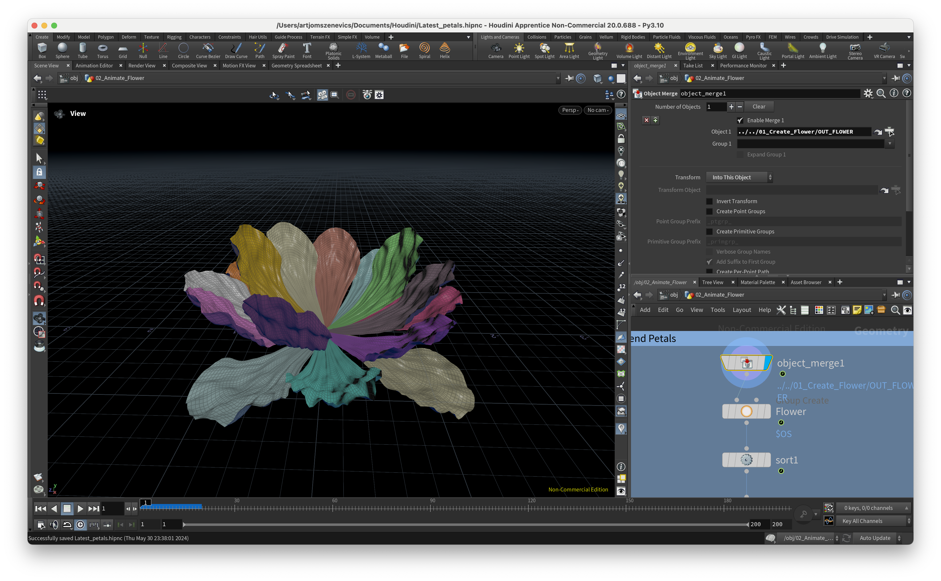
Let’s start by bringing the static flower asset from the previous Geometry object node into our new Geometry object, where we will be working only on animating the flower.
To do this, we need to use the “Object Merge” node and input the link for our static flower.
Step 2
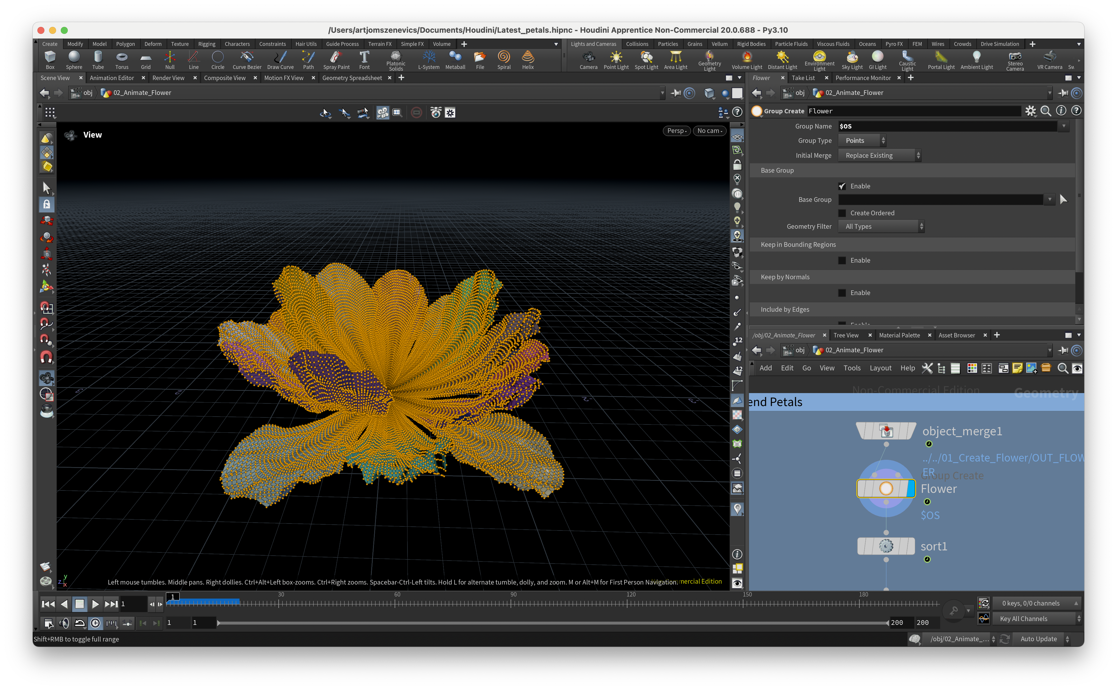
We’re creating a group of points from our object using the “Group Create” node.
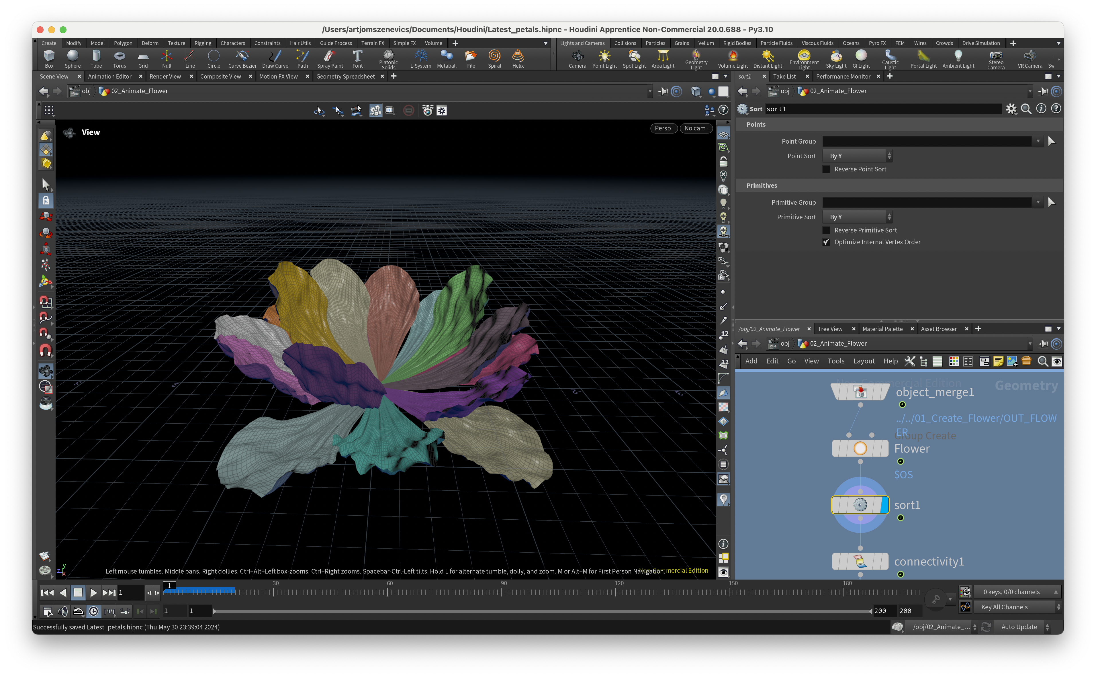
Step 3
The “Sort” node allows us to sort all the points and primitives of an object in different ways. In our case, we would like to sort them by the Y axis. This is necessary to ensure that the connectivity node will create a cloth attribute from the lowest to the highest petal. This way, the simulation will run in the right order.
Step 4
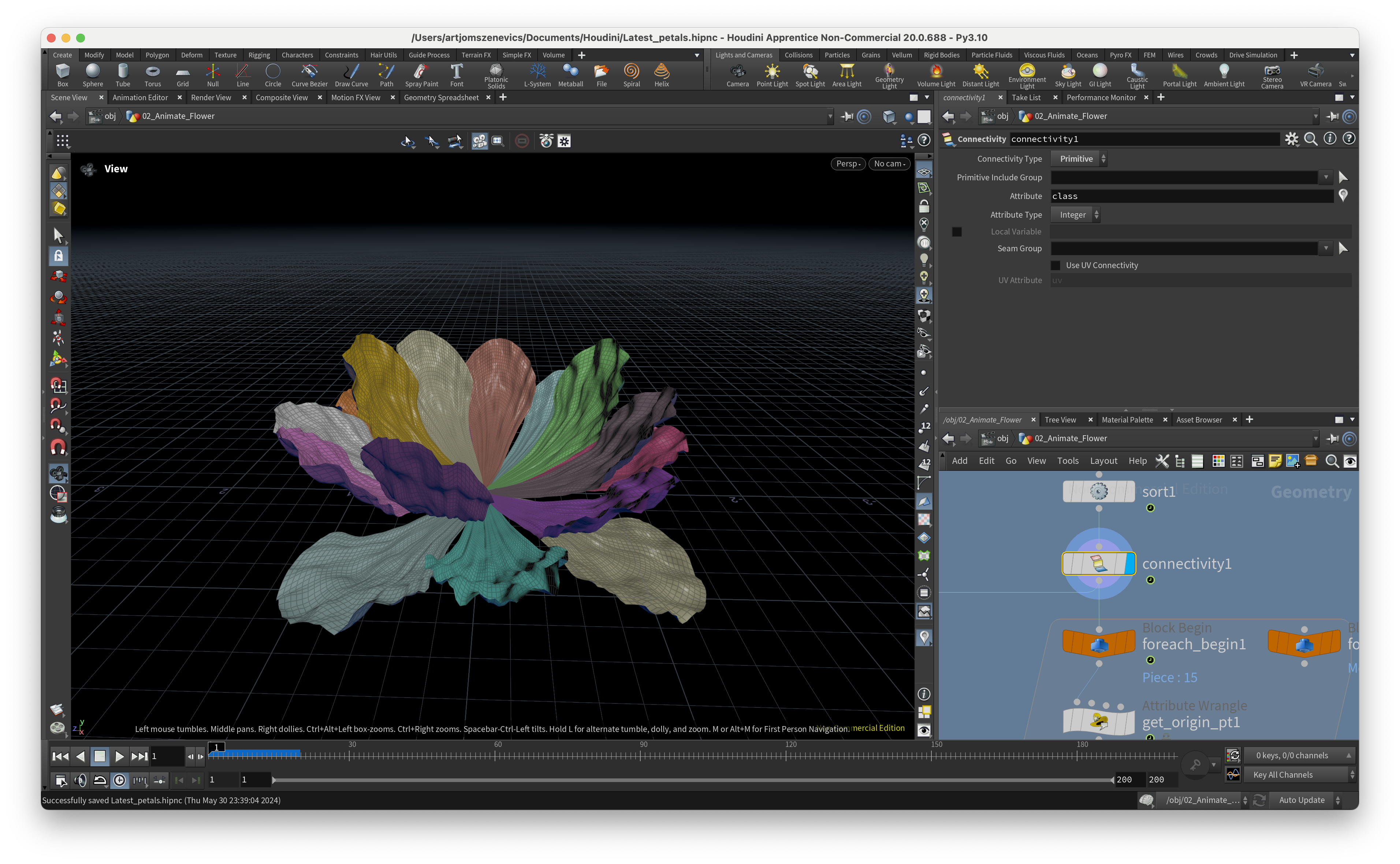
The “Connectivity” node allows us to have a unique attribute value on a set of connected primitives or points. This means each of our petals will have a unique attribute value. The default attribute name is “class.” We can use this attribute to count the number of petals and output this value to the Geometry Spreadsheet with the “Attribute Promote” node.
Next steps will mainly focus on the For Each Connected loop, which allows us to bend ANY kind of Petal one by one with the help of the “Bend” node. All thanks to procedural setup.
Step 5
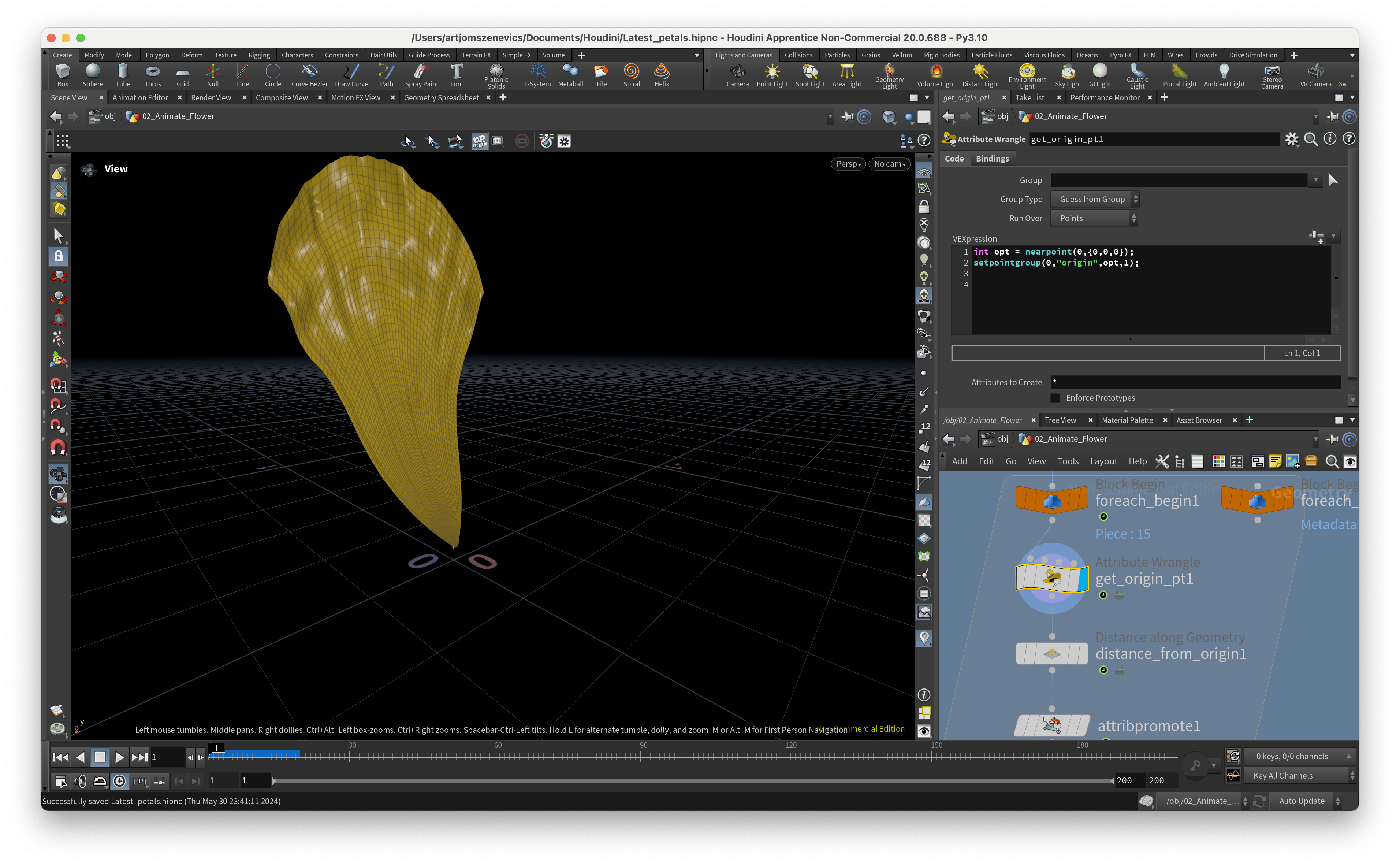
The first thing in the foreach block is the “Attribute Wrangler” node with this code:
int opt = nearpoint(0,{0,0,0});
setpointgroup(0,"origin",opt,1);
The “nearpoint” function searches for the nearest point to the world center axis. The “setpointgroup” function sets the point group named “origin” with the previously assigned variable “opt.”
Step 6
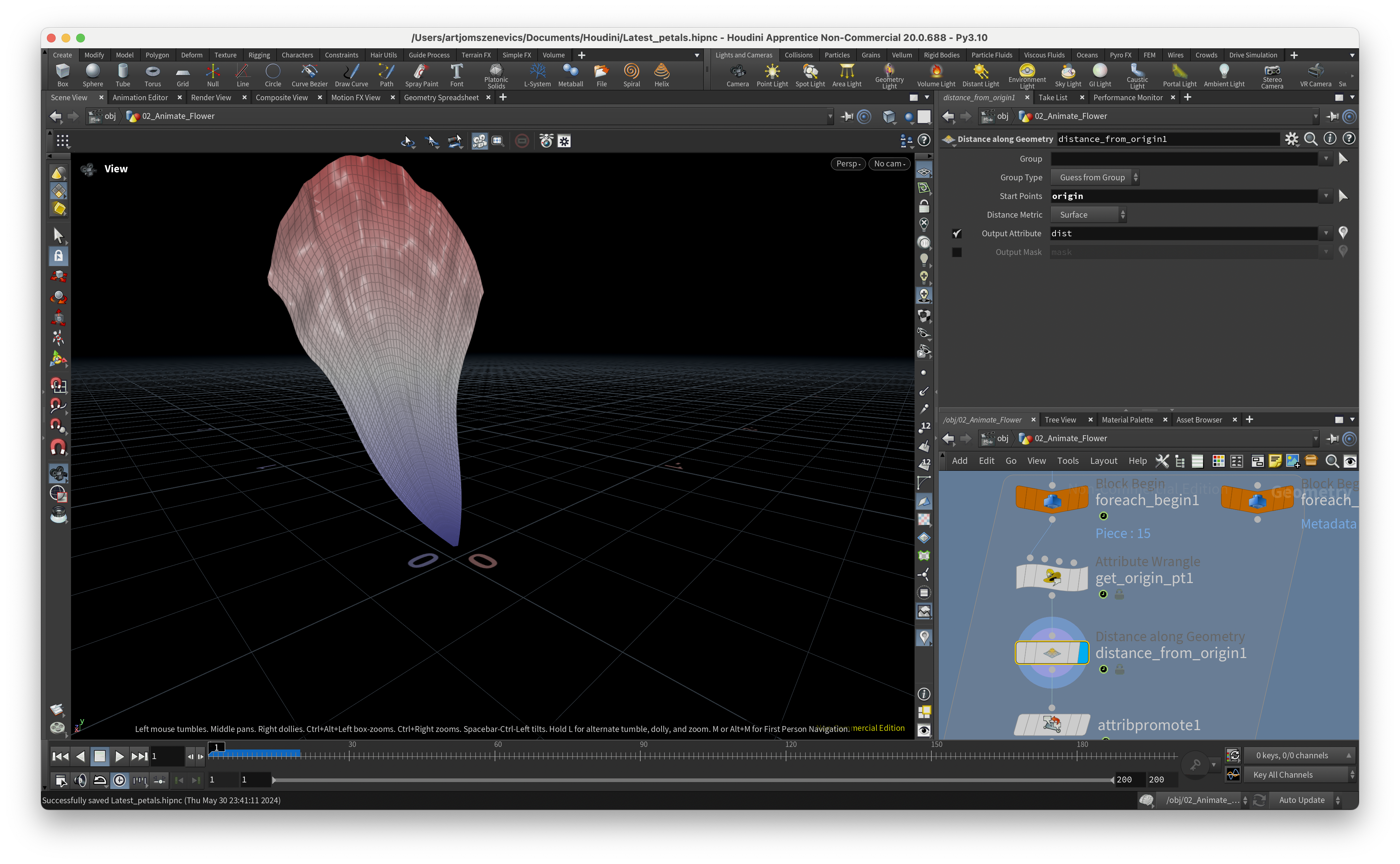
The next five nodes are interconnected, so it makes sense to go through them all at once.
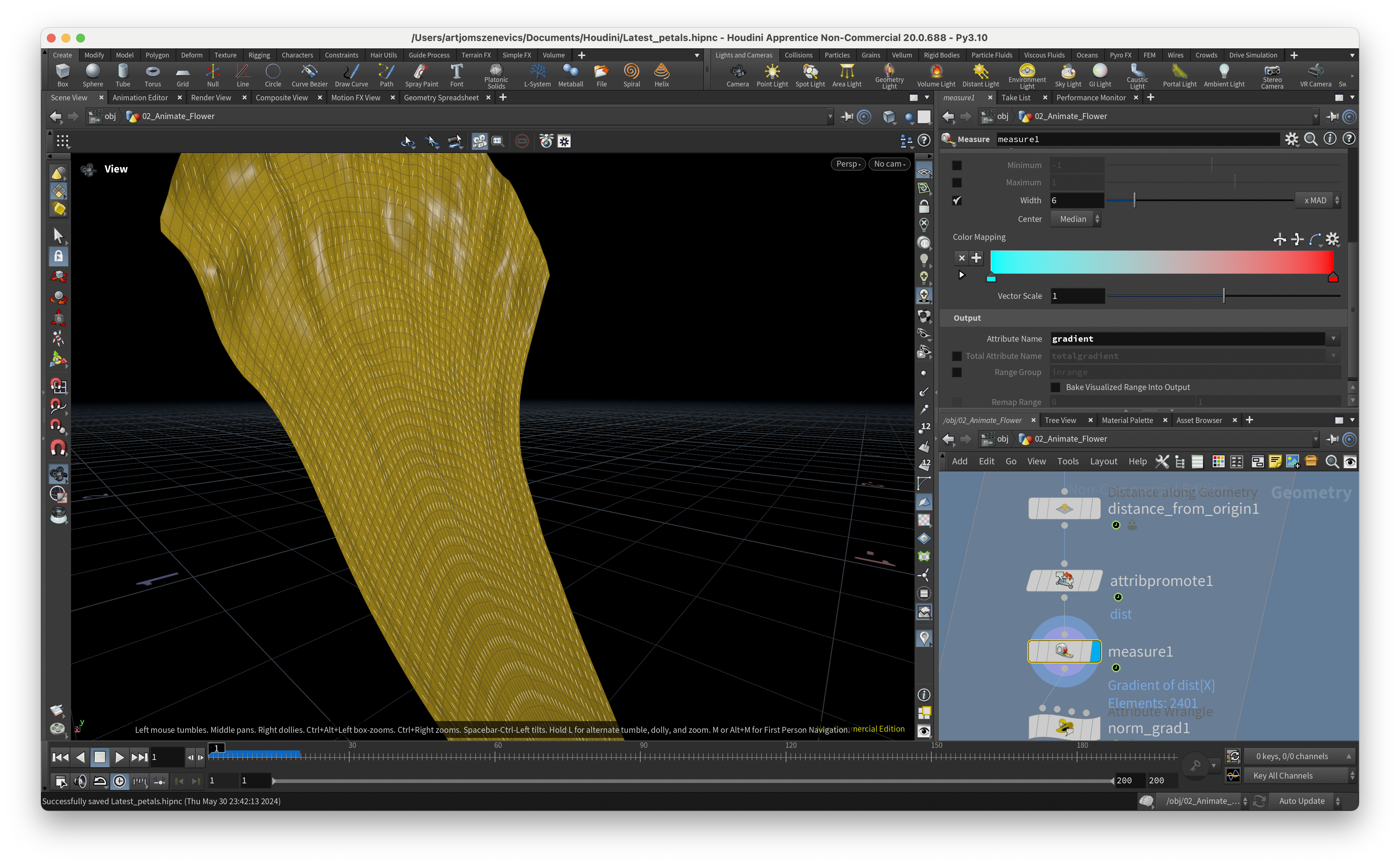
1. “Distance Along Geometry” Node - This node measures the distance along the surface, from our starting point to the end of the geometry. In the Start Points parameter, we use our previously assigned point group “origin,” and in the Output Attribute parameter, we place “dist.”
2. “Attribute Promote” Node - This node promotes “dist” from the Point level to the Detail level as a “capt_len” attribute. This value will be linked to the Bend node’s “Capture Length” parameter, allowing us to procedurally adapt our bend deformer length to different types of petals.

3. “Measure” Node - This node measures the curvature, area, or volume. In our case, we use the “Gradient” measure, which creates the direction across the mesh.
4. “Attribute Wrangler” Node - This node normalizes our gradient:
v@gradient = normalize(v@gradient);
A normalized vector means it retains the same direction, but its length is equal to 1, making it a unit vector.
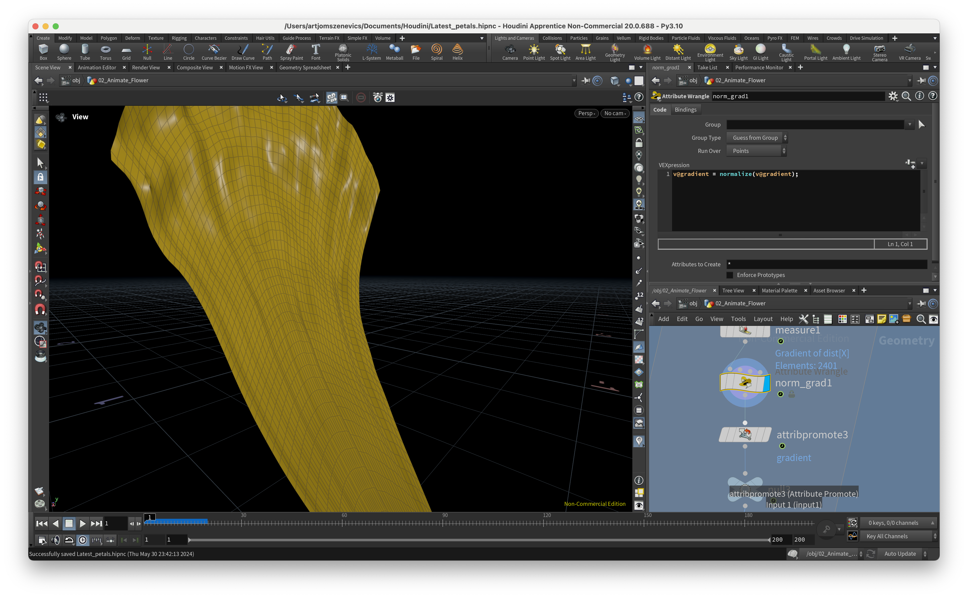
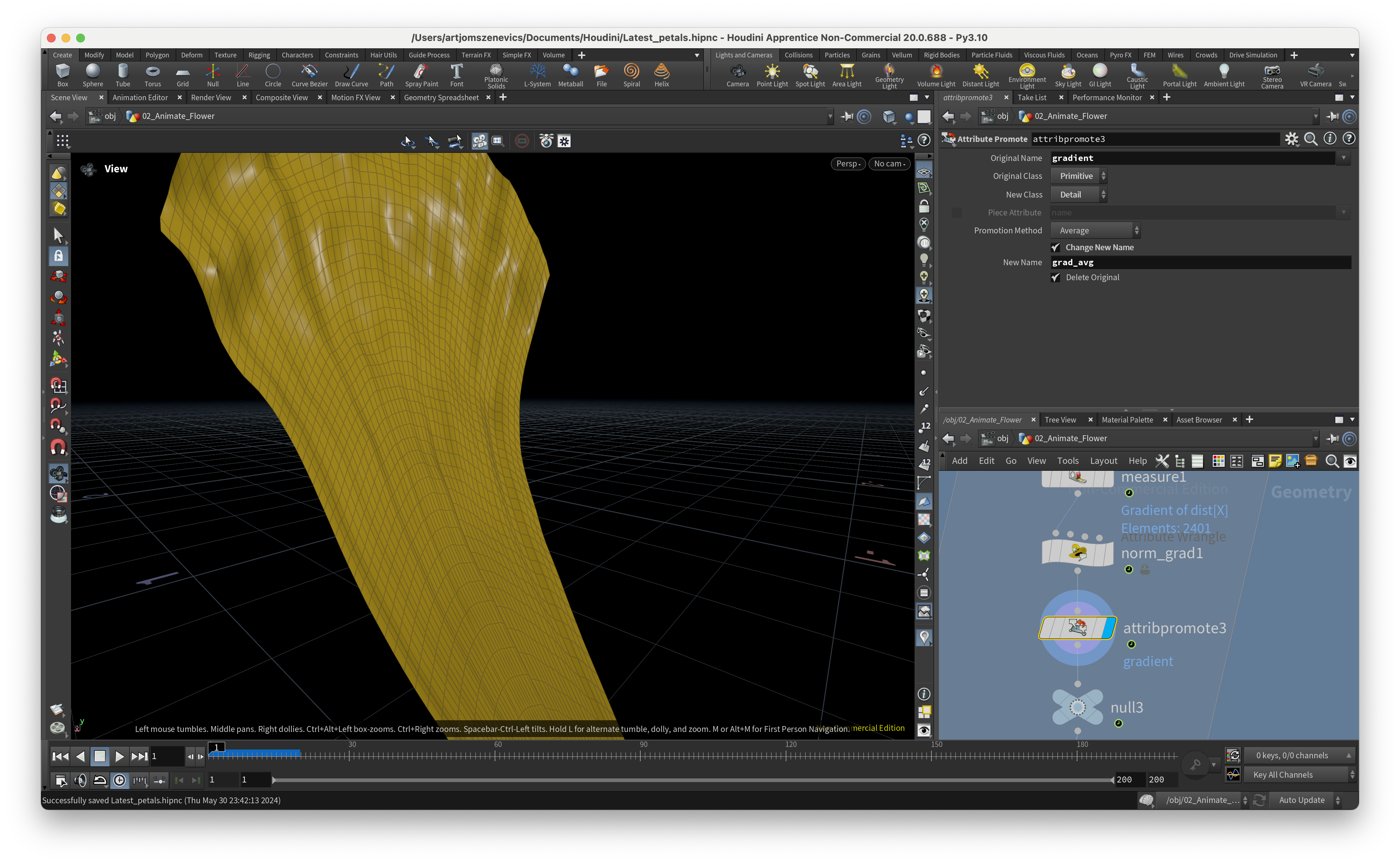
5. “Attribute Promote” Node - Similar to the second step, this node promotes the gradient from the Primitive class to the Detail class as the “grad_avg” attribute. We will use this attribute inside the “Bend” node.
Step 7
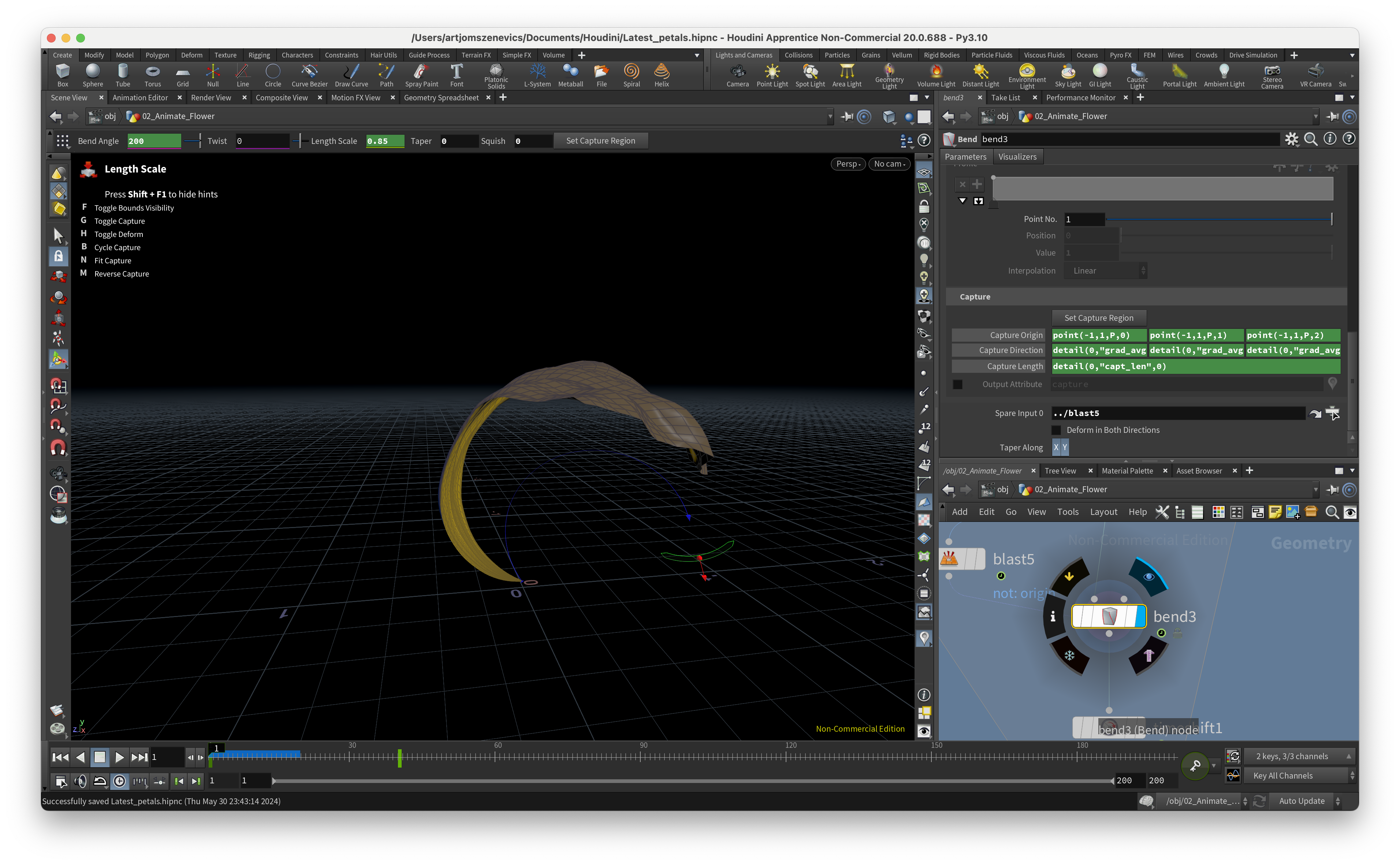
Finally, we use the “Bend” node, where we collect all our previously assigned attributes. The “Capture Origin” relates to our starting point, “Capture Direction” is the “grad_avg” attribute assigned using the “Measure” node, and “Capture Length” is the “capt_len” attribute assigned using the “Distance Along Geometry” node.
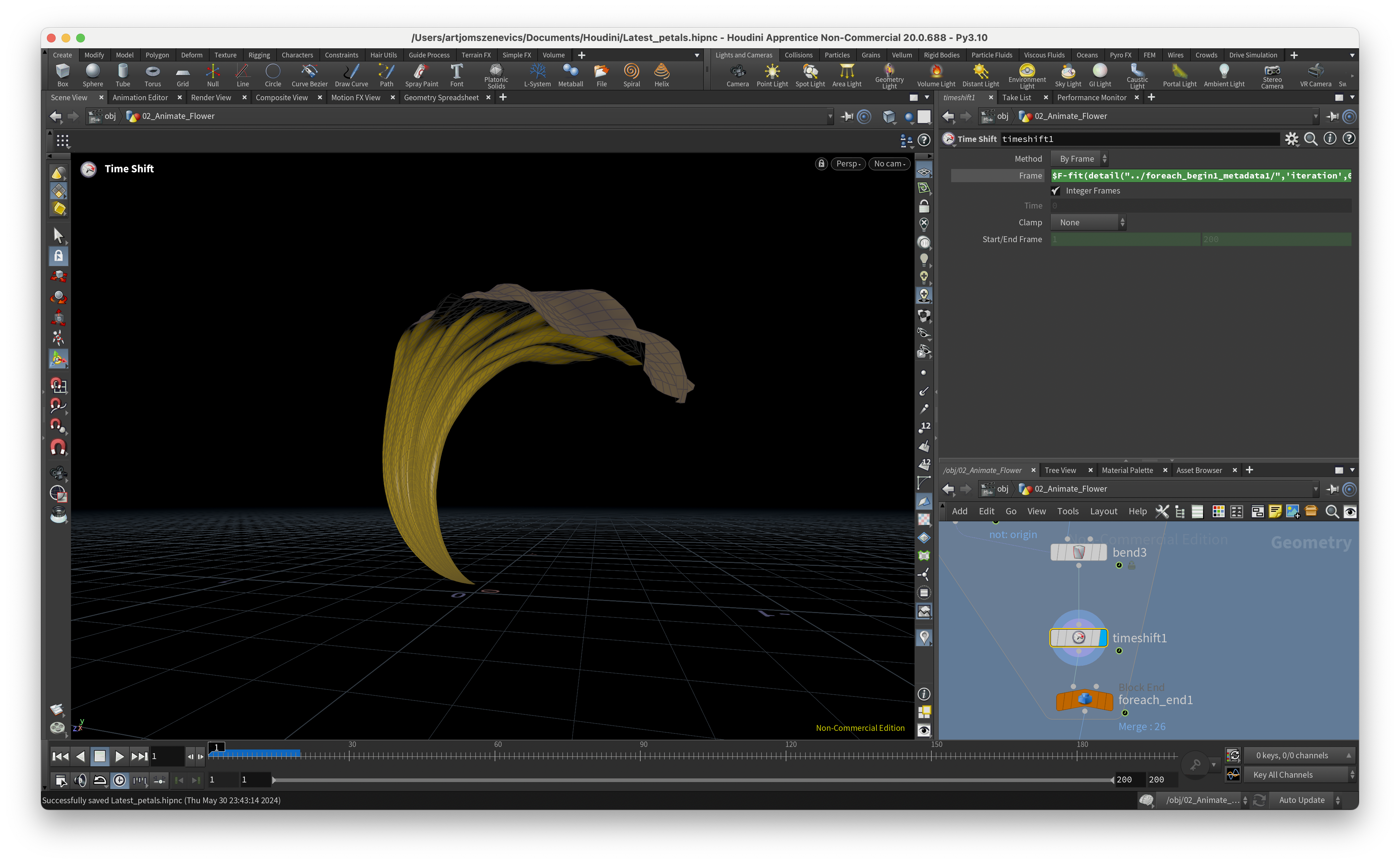
Step 8
The “Timeshift” node allows us to shift every petal by 40 frames using the fit() function inside the “Frame” input area.
$F-fit(detail("../foreach_begin1_metadata1/",'iteration',0), 0, (detail("../OUT_Num_of_Petals/",'class',0)+1), 0, 40)
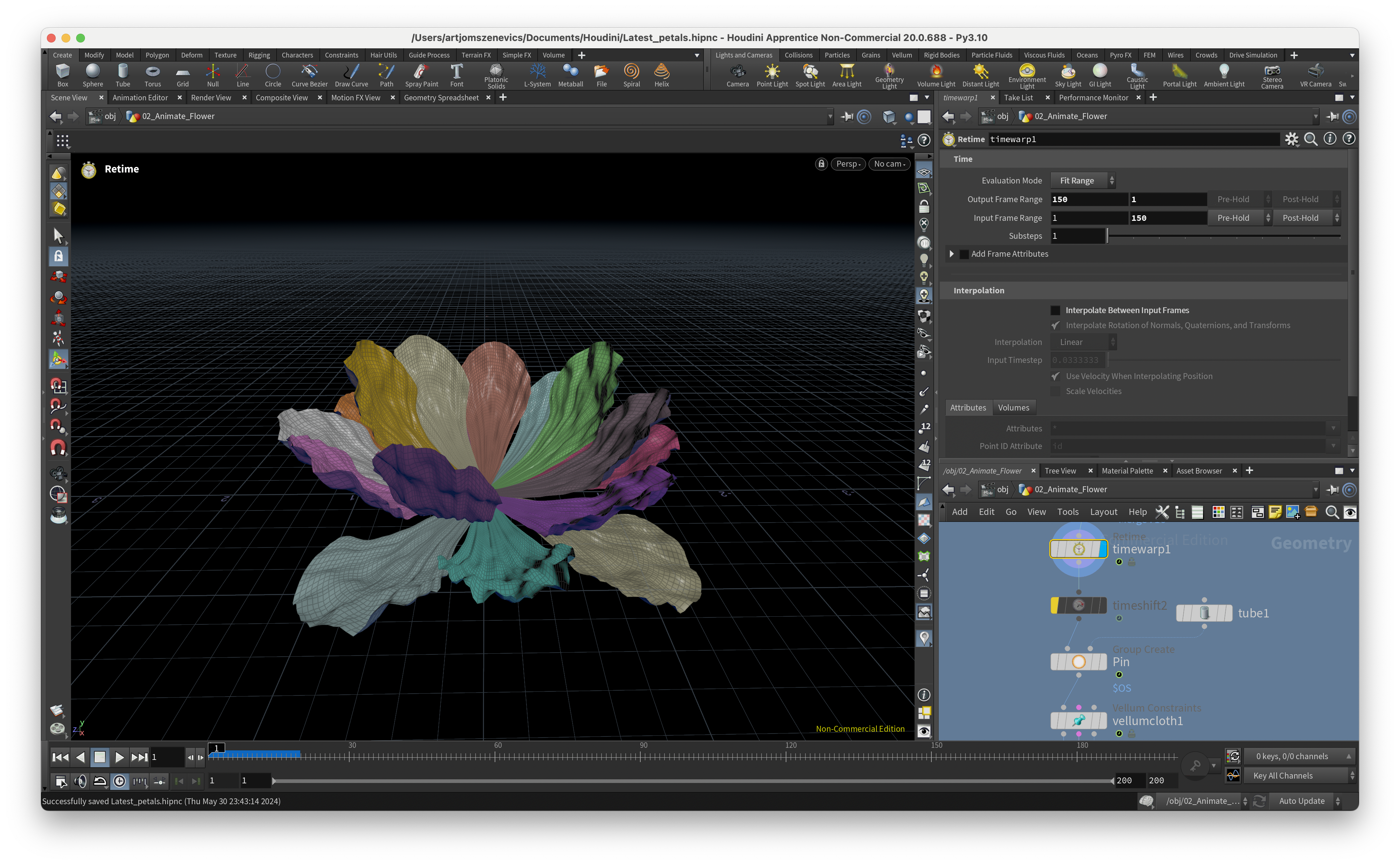
Step 9
Next, we continue to work outside the foreach loop and reverse the movement happening inside the loop by adding the “Time Warp” node.
The Output Frame Range is 150 - 1, and the Input Frame Range is 1 - 150.
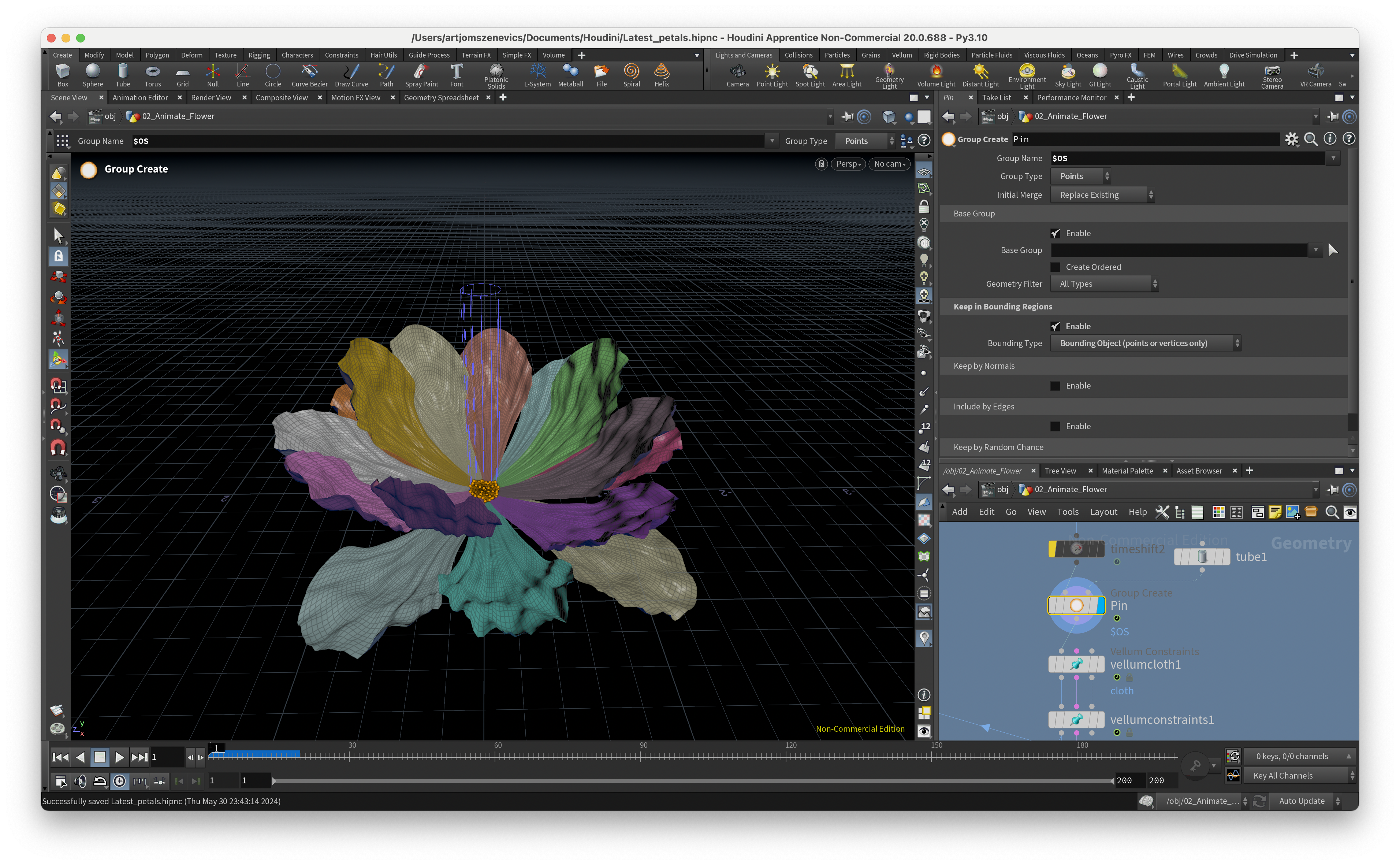
Step 10
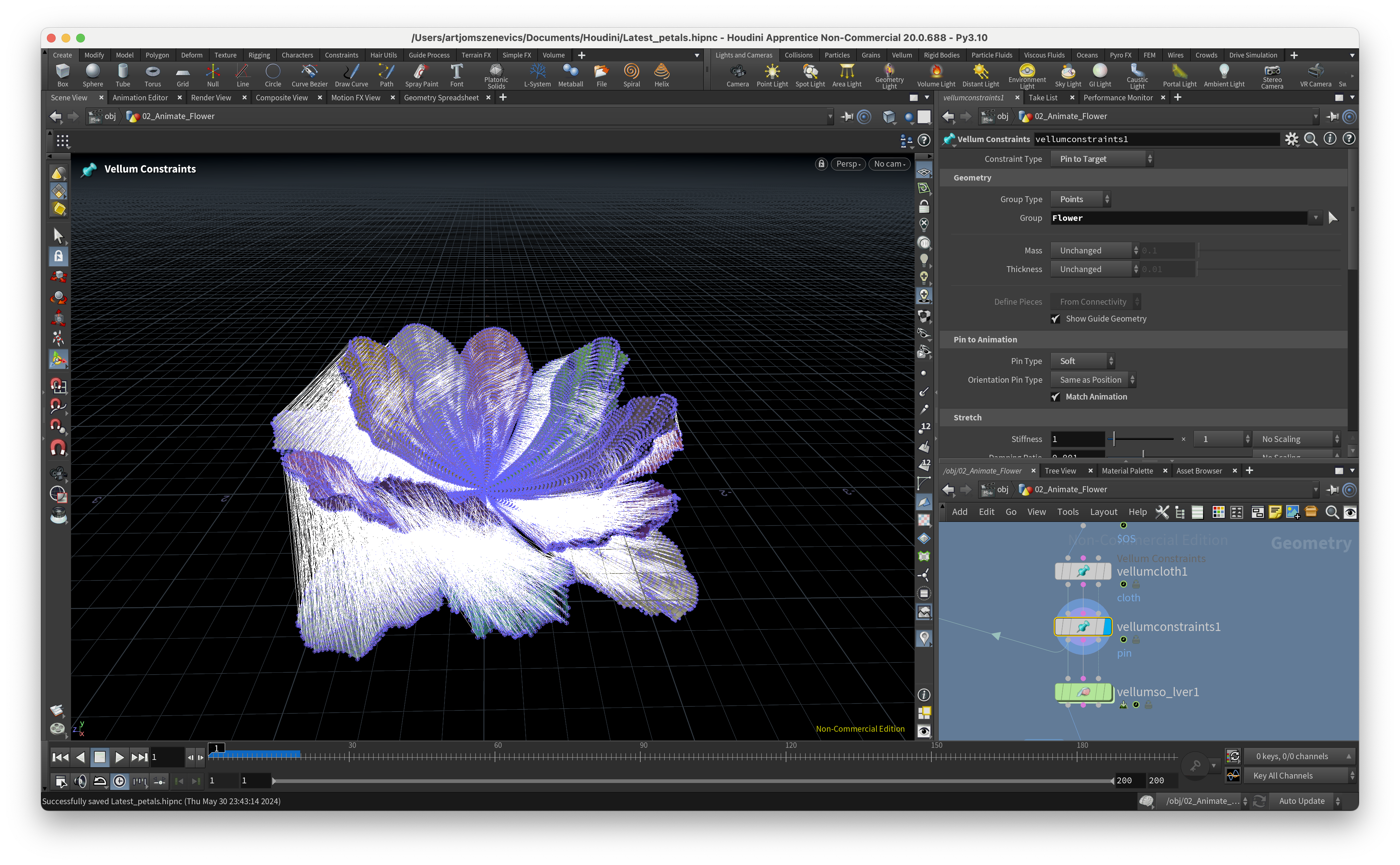
By adding a “Group Create” node, we create a point group that will act as a pin inside our “Vellum Constraints.” To include all the points of petals inside our connected tube object, we enable “Keep the Bounding Regions.”
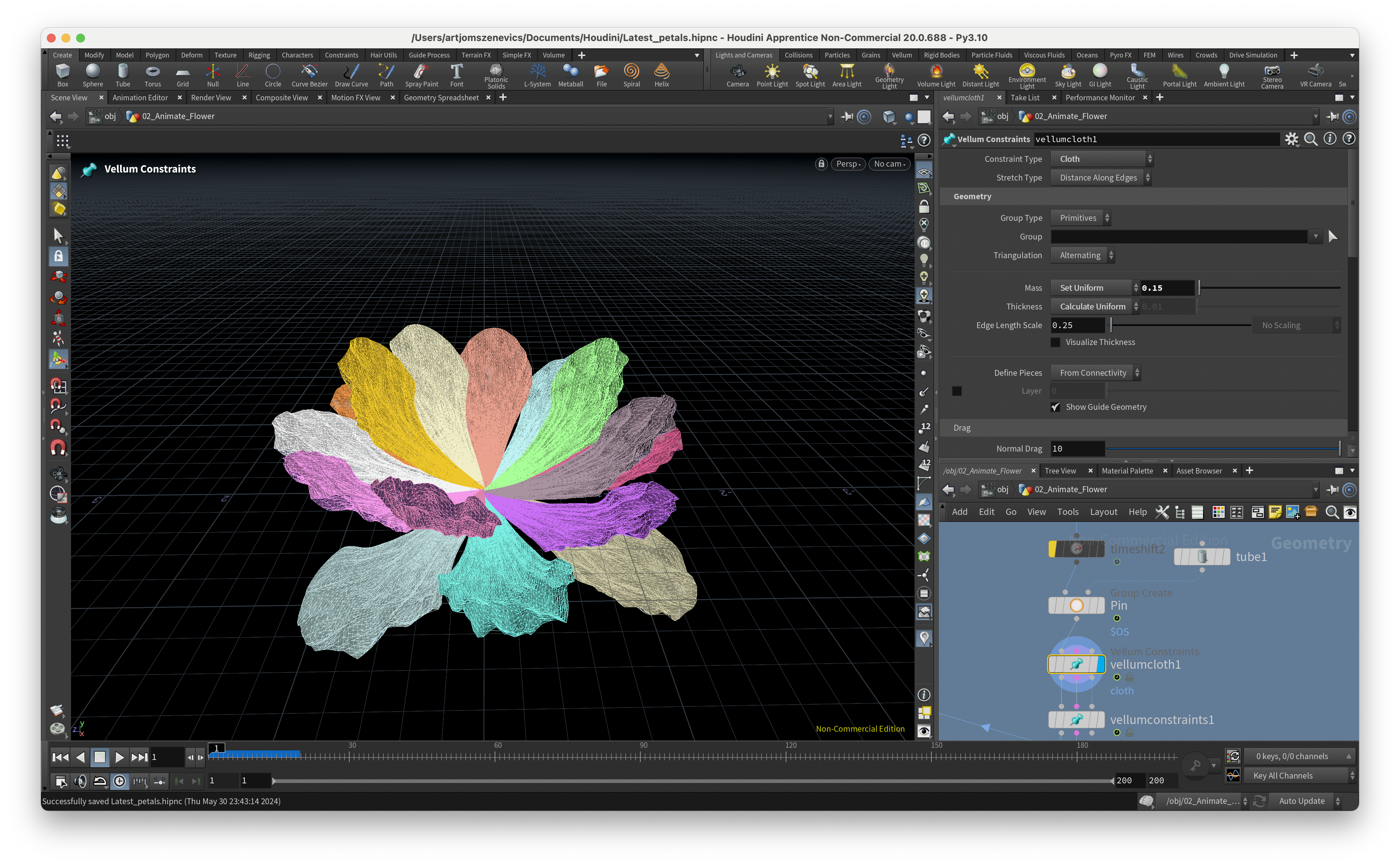
Step 11
The next nodes are fundamental for running any type of Vellum simulation, whether it’s cloth, hair, grains, or fluids. This is the main setup:
Vellum Constraints + Vellum Solver.
Paul also adds a bit of “Pop Wind” inside the solver to give the animation organic movement, simulating real-life wind.
Step 12
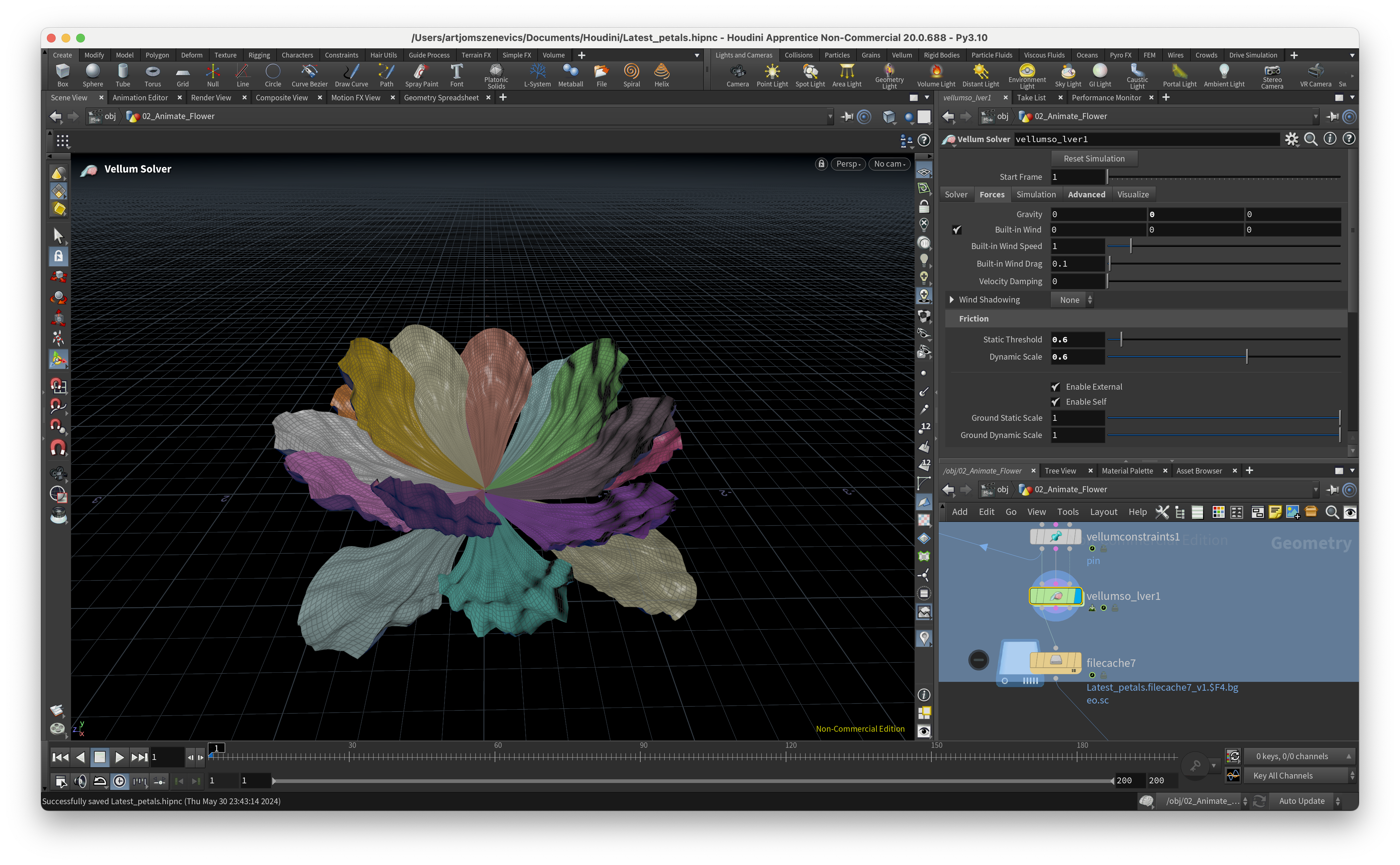
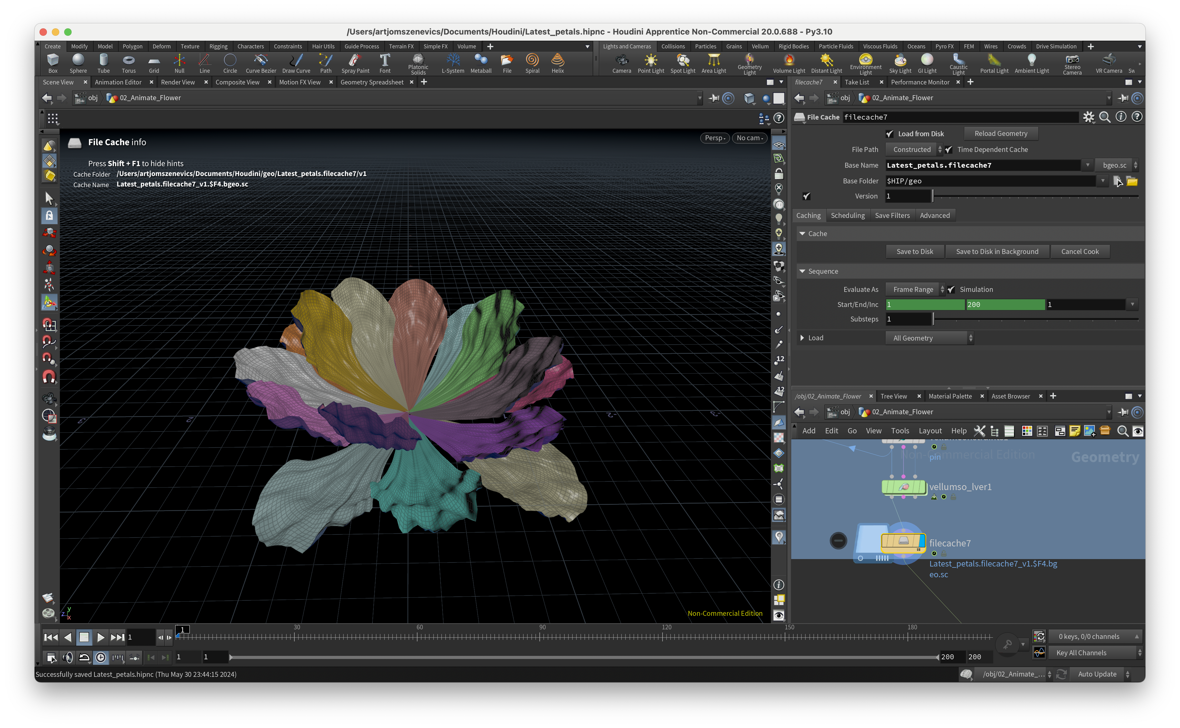
And last step for this article is to cache our simulation with substeps amount of 1 in Vellum Solver. Substeps is quite important because it will directly affect on simulation time. In short substeps is the amount of how much the simulation is going to be re-calculated per frame.
Conclusion
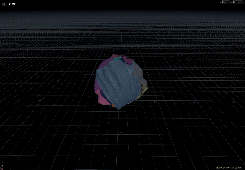
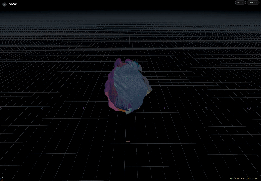
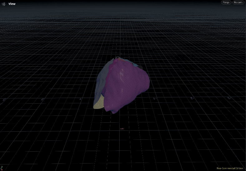
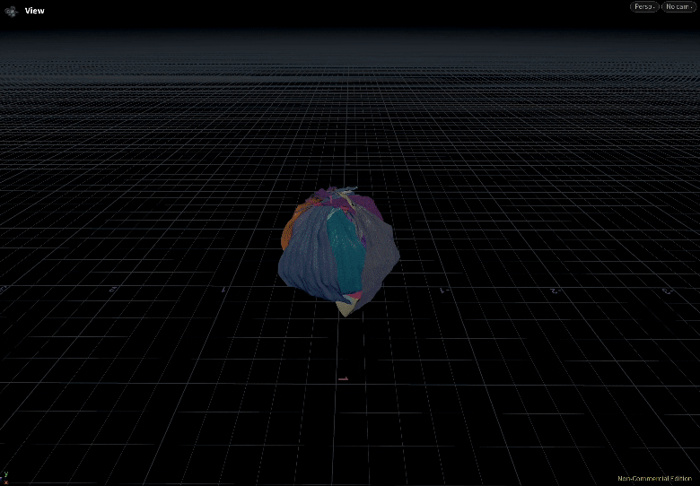
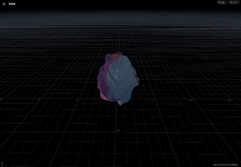
In the end, I spent a lot of time getting the right simulation and adjusting the settings of the Vellum Constraints and Solver. However, the default settings also worked fine. Below, you will find a few of my simulation tests using previously created petals. As you can see, not all the simulations are accurate due to incorrect geometry input into the solver.
Geometry needs to be clean and non-intersecting with each other on the input. Otherwise the Solver will end up in geometry errors.
Next on my plan is to combine everything together: the petals, stem, and pistils as one complete object.